ArduPilot Linear Quadratic Attitude Controller
You’ll be most interested in this post if you’re interested Ardupilot (See Ardupilot dev info). If you’re not interested in ArduPilot you might still appreciate the next section that covers basic software architecture for any system such as this.
In this post we’ll cover how a linear-quadratic (LQ) attitude controller replaces the ArduCopter native PID controllers for the independent roll, pitch, and yaw axes in the copter code.
High-level software system architecture
Before we get into specific Ardupilot software implementation for our attitude controller let’s pretend we don’t have any software and need to think about how we’d start from scratch. How would one generally architect a control system software scheme to control the position and orientation of an object like a quadcopter?
Position is the X,Y,Z location of some object’s, “control point”. For us it’s the mass-center of our quad: the point about which roll, pitch, and yaw rotation occurs. Orientation implies the direction something is pointed, and depending on degrees-of-freedom this is more-or-less complicated. For example, a ground vehicle on a flat surface is typically restricted to compass heading (comparable to our yaw). However, in the air we add roll and pitch and we refer to this as, “attitude”. It implies roll, pitch, and yaw.
This means we desire to control six degrees-of-freedom: X, Y, and Z relative to some ground reference as well as roll, pitch, and yaw of the body relative to the ground reference frame (typically North, East and Down/up. or NED)
Where would we start from scratch?
Starting from scratch we’d assume we’ll take ground control inputs (joystick, waypoint upload, etc). We know we’ll have sensors on-board (inertial, magnetic, altitude, airspeed, GPS, and so on). How do we layer all this into a workable system?
Software architecture concept
This is by no means a complete sketch or list that follows the diagram below. It provides a simple view of how a control system like ours needs to operate with various layers of control and through various sub-systems.
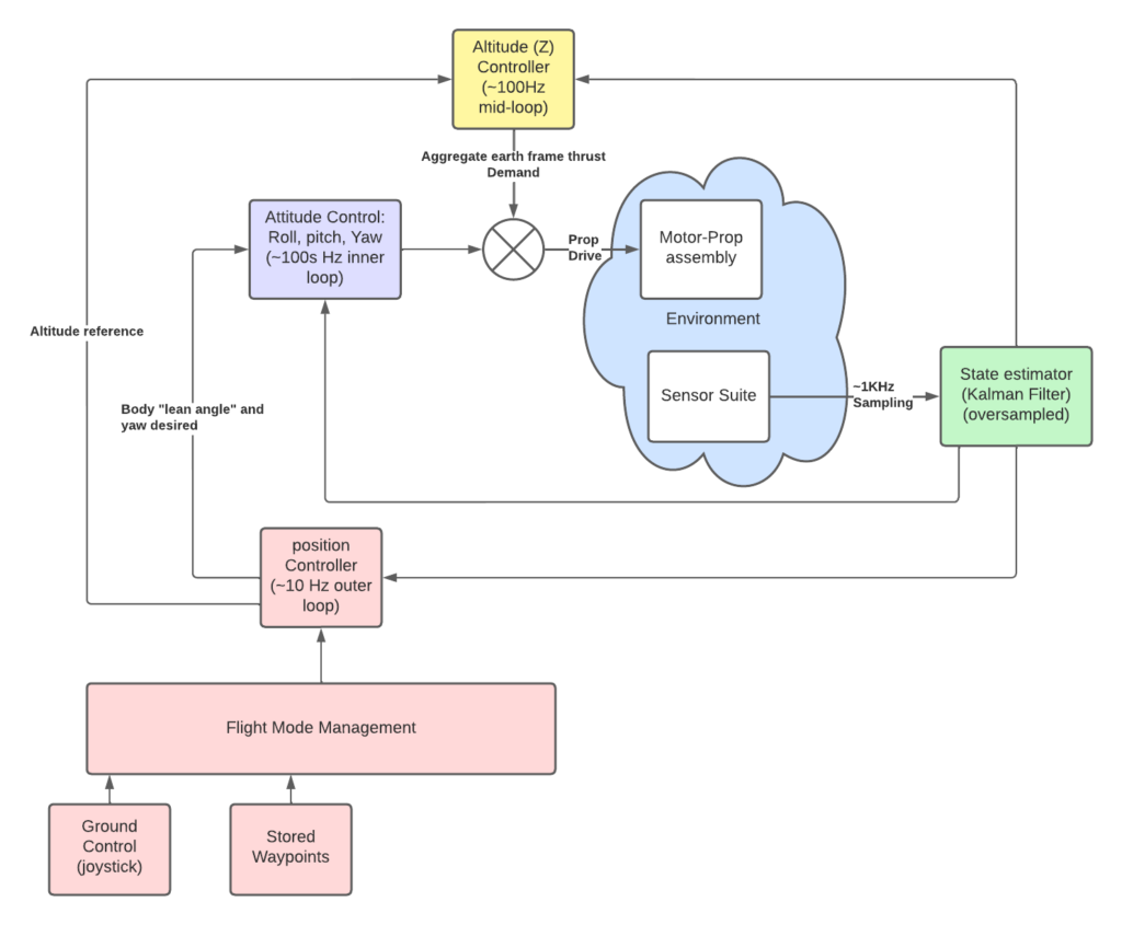
The diagram above covers this high-level concept for layering-in our software.
- Assume you’ll be fast-sampling your sensors and running a “state estimator”
- Assume this is going to run at a fairly high rate (relative to plant bandwidth).
- It’s going to perform all the sensor combining (fusion) to produce…
- “clean” estimates of state information for the slower running control loops
- A, “state estimator” can be as simple as an averaging scheme on single sensor…
- or something more complicated like a Kalman Filter for many states.
- Whatever it entails, it’s where the control loop gets it’s (cleaned-up) sensor data from.
- The fast (inner) loop will control attitude relative to reference.
- This needs to operate 5-10 times faster than the bandwidth of body rotations about it’s mass center
- Outer position loop is going to provide reference roll, pitch, yaw.
- The current state is sampled from the state estimator above.
- Attitude error is difference between reference and current state estimates.
- Apply our, “control law” (gain on the error)
- Condition command output for a motor drive action.
- repeat “inner loop”…
- A slower-running loop is controlling Altitude relative to position and…
- As part of position loop below or intermediate to the position loop.
- Gravity is always acting on our craft and we need a Z-controller to keep aggregate vertical thrust maintaining altitude to desired reference.
- An outermost (slowest) position or “flight control” loop
- This is operating 5-10 times faster than the bandwidth of the center-of-mass of the craft.
- This is slower than the attitude bandwidth.
- This is where either manual (joystick) inputs are fed directly or…
- waypoint or other mission logic is processed into position errors and…
- required attitude (lean angle) reference inputs to the inner attitude control loop.
- This is operating 5-10 times faster than the bandwidth of the center-of-mass of the craft.
Rough technical requirements we can estimate up-front
Given a basic architecture concept above, before we’d write any code we’d be able to estimate that a Kilogram-or-two mass (heaviest element being a battery pack) is going to have roughly a 10Hz bandwidth. Rotations of that body with low-mass motors on arms will have a bandwidth still higher, say 10’s of Hz.
This immediately informs our design and gets us to some estimates for technical requirements. Conservatively, we know we’re going to need to operate at the following orders-of-magnitude…
- Sample sensors near the 1KHz range
- Run our attitude controller at 100+ Hz
- Run our Position and controller (and altitude) at 10+ of Hz
You can always run a sampling-and-control loop much faster than you need to but it implies over-design of hardware and real-time software architecture.
There is a convenience to some over-sampling (faster than technically necessary) loop design: you don’t need to consider discrete effects, typically (We’ll cover continuous and discrete design concepts later).
With a mechanical system like our quadcopter we can come to the above estimates by instinct and experience, and know roughly what our hardware and software is going to need to to by way of sampling rates and control loop frequencies. However, in our case ArduPilot has this all framed-up!
Ardupilot Implementation
This section will be most interesting to readers interested in working with the ArduPilot codebase.
Fortunately for us we don’t need to architect and code-up a complete system to get our Linear Quadratic Attitude controller into action!
Ardupilot has all the sub-systems in-place for us. All the, “loops” and their timing touched-on above is implemented. We’ll also be able to start by taking advantage of the resident Kalman Filter (State Estimator in the basic diagram above).
We’re going to dig into the implementation of our new attitude controller and get it controlling stable roll, pitch, and yaw in a simulated environment on the bench.
Existing ArduCoptor AC_AttitudeControl_Multi logic
ArduPilot’s ArduCoptor code uses a class named AC_AttitudeControl_Multi to implement attitude control for quadcoptor. You can read about the resident implementation here. The basic design involves three independent (uncoupled) PID controllers to control to roll and pitch, “lean angles” and body yaw.
Outputs from the three PID’s scale a -1 to +1 range for a next-layer-down motor code object that takes these unity ranged values as “set_roll”, “set_pitch”, and “set_yaw”.
We need equivalent -1 to +1 values scaled from our LQ controller’s roll, pitch, and yaw command torques to set to the motor object.
New AC_AttitudeControl_Multi_LQ
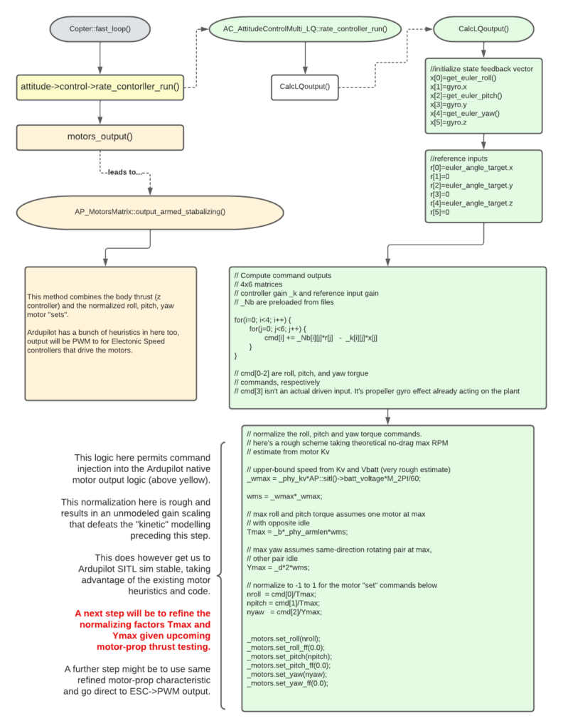
We replace the native attitude controller with a new one: “AC_AttitudeControl_Multi_LQ”. Below is a stripped-down diagram and pseudo-code illustration. The “fast_loop” into yellow blocks is unchanged code flow. We just have that “rate_controller_run” call-in to our replacement attitude controller.
Within this, you can see the code is as simple as…
- Read state estimates into the current state vector ‘x’.
- Set reference input state to the desired “lean” angles (euler_angle_target)
- x,y,z here implies roll, pitch, yaw (this is just Ardupilot vector notation).
- Our Reference and feedback gain matrices ‘Nb’ and ‘K’ are pre-loaded.
- For now we’re keeping them constant:
- As described here we can evolve this over a more dynamic flight envelope.
- We’ve zeroed body inertial effect on state transition matrix, A.
- We’re ignoring propeller gyroscopic effects in matrix B.
- As described here we can evolve this over a more dynamic flight envelope.
- For now we’re keeping them constant:
- We operate on our reference-minus-current state error with our gain
- Last step is to normalize torque command outputs into -1 to +1 Ardupilot motors inputs
- Were’ going to refine this in the next post.
Results: Stable on the bench!
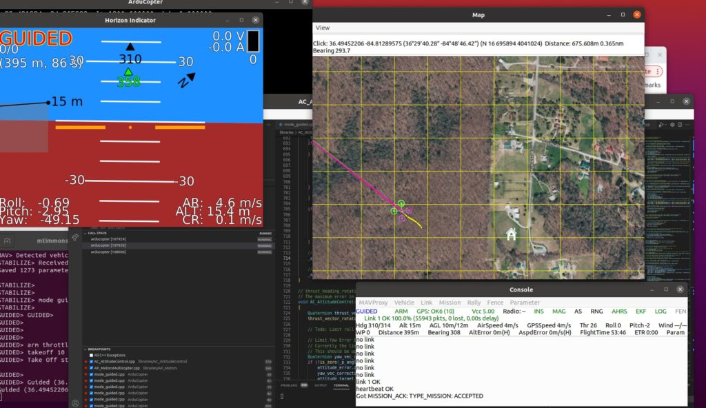
We can go into more depth later on how to run ArduPilot against a simulated vehicle. For now the screen-shot below shows our little quad stable on-screen. See Ardupilot Software-in-the-loop (SITL) documentation for a description of how we’re running the controller in software against the simulated Matlab copter descibed in the video below.
- Takes-off to stable altitude and attitude.
- Yaws to a screen-clicked, “fly to” point and proceeds to converge on the new waypoint.
- This involves the native position controller feeding yaw, “lean angles” to the attitude controller.
- Attitude controller takes these reference inputs.
- operates on state errors with gains as detailed above.
- Outputs to motors as above.
Ardupilot simulating our stable Linear Quadratic attitude controller
Short video describing the “Software in-the-loop” (SITL) Matlab Simulator
See Ardupilot Matlab SITL for details and resources, including the Matlab code shown here for simulating the EDU-450 platform.
Our LQ Attitude Controller simulating against the Matlab vehicle
Here’s a screencast of the ArduCopter code running the LQ attitude controller detailed above.
You can see we’re stable on takeoff to hover and also on a fly-to a new waypoint. From there it’s a bit rough as it hunts around the new point. This is some interplay between the position controller and scaling errors around the desired point. We’ll figure this out.
This LQ scheme is actually quieter in the horizon display than the native PID scheme because the SITL sim vehicle parameters are baked-in to the LQ scheme’s kinetic model (The A and B matrices).
This makes the sim pretty quiet, but in the real world we’ll have other problems and it won’t be this neat. For example, bias errors might yet require us to integrate out attitude errors. For now, it’s good to be simulator-stable. We’re on the right track!
Conclusions
Being closed-loop stable with the simulator is a big step! We’re not flying yet, but getting our attitude controller wedged within the Ardupilot position and motor code took some wrestling and learning to figure out. To be simulator-stable means we’ve got the proper code, signs, and data relationships figured out!
Next Up…
Our command torque normalization to -1 +1 for input to motors is rough. The hack method in the flowchart above got us stable on-screen but it won’t fly (pun intended).
We’re going to characterize our motor-prop assembly for actual maximum thrust and use this as our normalizing factor instead of the computed method above.