1

Quad-Rotor Control Design Series

What is a “quad-rotor”? Well you probably know it’s a thing with four rotors. We buy it as a, “drone” and we fly it with a remote control or via a phone app acting like one. I’ll probably bounce between the terms quad-rotor and quadcopter throughout. I mean the same thing. It is incredible what we can buy today for fun, and not too much money. Camera technology is awesome too.

I chose this gadget for a deep-dive because these things are popular. We can all remember seeing one fly, or maybe you own one. A quad-rotor is also a great example of a multi-output control system with multiple sensor inputs as feedback (MIMO system). We can go from simple to very complicated design ideas using this common vehicle as a platform for study.

How a Quad-Rotor Moves In the Sky

When you command a commercial quad-rotor drone to move up, down, right, or left relative to where it is in the sky, the machine processes that, “command” relative to the current location. Then it changes the speed of the propellers in such a way that the drone will move as you desire. A simple way of understanding it is as follows…

  • Two pairs of Propellers, opposite each other on the two arms that intersect at the center.
    • One pair rotates clockwise (CW – green above)
    • The other pair counter-clockwise (CCW – blue above)
  • Imagine driving one propeller of the green pair faster than the other green one.
    • if we left the blue pair equal, the body of the quad-rotor will rotate about a line between the two blue propellers above.
    • Same logic applies if we do the same to the blue pair, leaving the green equal: it will rotate about a line between the green propellers.
  • If we vary each pair more-or-less simultaneously we create a more complicated tipping action of the platform, but it’s basically just doing as described above to create a, “virtual” axis of rotation

One last motion: Yaw…

  • There’s one more less obvious motion: making the entire body we see above rotate about an axis coming out of the screen. This is, “Yaw” for this platform.
    • This relies on the counter-acting torque on the body of the quad-rotor as a result of the drive torque on the propellers: It’s Newton’s Third Law stating that for every action there is an equal and opposite reaction.
    • Here’s a way to visualize it for a single propeller. The plane wants to rotate the opposite direction. For a single-engine craft like this, the ailerons and rudder work to cancel this out.
    • The quad-rotor has four propellers. Here’s how we can make the quad-rotor, “spin” like a figure skater while remaining otherwise stationary
      • let’s say we start in a fixed spot in the sky, level, and not moving: hovering still.
      • If we speed-up the blue propellers above just a bit, and slow down the green just a bit so the total, “up” thrust is otherwise still the same…
        • the little extra reaction torque on the body of the quad-rotor by the fast propellers compared to the slower propellers will cause it to spin one way.
        • If we flip it around and make the green a bit faster, the quad-rotor will yaw the other way.

No matter what the current roll, pitch, or yaw angle is at a given moment, if we increase or decrease every motor drive torque by the same relative amount the entire machine will move along the vertical axis of the drone, in theory.

Complications…

There’s a lot going on relative to non-linear propeller drive force equations, wind, and gyroscopic effects perhaps. The above explanation is simple enough for understanding the basics, but we rely on sensors to continuously measure and feeedback to the body controller so it can update the propeller speed controllers. This occurs very many times per second.

The presentation below does a good job of introducing the sensor concepts, and covers much of what I will likely repeat, but I am going to go into some more detail in a few areas to cover how to derive some of the equations, how to simplify the model to the degree shown here, or maybe not simplify it.

Also, this presentation looks to cover the simplified modelling and control using Proportional-Integral-Derivative (PID) controller pairs that act independent of one another to control pairs of propellers relative to, “level” flight. That’s a fine and robust simplification for a stable camera-drone platform.

I’m interested in learning what it would take to control one of these things over severe bank angles, or a larger, “flight envelope” so this topic is going to take us into a lot of details and learning. Can’t wait to get into it!


QuadCopter Dynamics and Controls: Ramp-Up Reading…

I started to sketch a quadrotor model myself and derive the equations of motion, but I lost confidence and figured it would be best to sample the literature first. Below is a list of papers I found online. Click the links to see the papers.

All the papers are useful, but I found the, “PID vs LQ Control Techniques Applied to an Indoor Micro Quadrotor” by Bouabdallah et al. to be a most useful reference. It is becoming my primary basis for understanding and modelling the system I need to design a controller for.

PID vs LQ Control Techniques

modelling_of_quadrotor_minicraft

design_of_four_rotor_aerial_robot

Thesis KTH – Francesco Sabatino

State Space System Modeling of a Quad Copter UAV

Modelling of the ETH Helicopter

linearization

A goal here is to develop a dynamic model and controller scheme as a platform for learning and applying, “Optimal Control and Estimation” techniques.

The multi-input model can be broken into a set of independent PID servos for level flight (hover). It will be interesting to retain the coupled system in which roll, pitch, and yaw terms interact over a larger, “flight envelope” (larger roll and pitch angles) and not just small control action from level flight. It might not be necessary for much practical flying, but we’re going to follow some advanced topics for the fun of it.

The Bouabdallah paper above doesn’t jump to model simplifications and linearizations. It maintains consideration for gyroscopic effects because the focus is on a lightweight, presumably highly dynamic platform. I’m also intrigued by the, “successive linearization” concept presented.

We’re going to get a better grasp on model linearization through this exercise. We’re going to better understand how to modify the, “state transition matrix” (typically termed matrix ‘A’ for continuous control models and ‘F’ for discrete-time models). Hence the, “Linearization” paper above.


Dynamics and Controls Study Materials

I’ve enjoyed great opportunities to both study and work on mechanics, electronics, real-time control systems and supporting software for automated machines: Agricultural machine control for the most part, and some neat control systems problems in communications, sensors,  and other areas.

Dynamic Modelling

One thing I really like about, modelling a dynamic system is you need to be creative to arrive at an appropriate model, or mathematical representation of a system. It is just like a scale-model in that it isn’t the, “real thing”. It is something that represents the actual system, in a form simple enough to apply some math to, but not so complicated that you can’t solve the equations into some control electronics and software.

This modelling step is my favorite part. It is the most important part. If it’s too complicated I can’t work with it. If it’s too simple, it means I’m probably ignoring something in the real world that would make any system design fail to do the job correctly. There really is not much math at this point, but a sketch and an accounting for what goes in, and what goes out: the stimuli you expect to make the system do it’s work, and also the forces of nature that want to move the system in ways you can’t always know, but need to manage somehow.

Differential Equations Comprise the Model

Because we’re dealing with dynamic systems we’re talking about differential equations to represent them. This just means an equation that describes, given where something is (it’s current state), where it is going based upon some attributes and some forces acting on it right now.

It’s kind of like this: if you know where you are standing, you know how heavy you are, and how strong your kid is who is trying to push you out the door to drive him to a friend’s house, we might know how much closer to the door you will be one second from now.

These Differential equations are the mathematical model of a dynamic system. At this point of our model they might be too complicated for us to do much with, so we might need to decide if there are terms we can ignore because they will have a small effect, or maybe we need to linearize the system by making some assumptions about the range of action (motion) we expect relative to perhaps a typical operating point.

Creativity

Proper simplification requires creativity. There are so many great examples of similar problems (especially now with the vast resources of the internet) that it is fun to borrow techniques and sometimes combine techniques from different problems to a problem at-hand. The best ideas are typically stolen.

In order to be creative and confident in our modelling of the Quad we’ll need a solid foundation. Here are some references I often revisit.

Control Systems Basics: review of the old studies

This is introductory Controls textbook.

This is introductory Discrete-time controls text that builds on the text above. Most controllers today are implemented by a digital computer that samples sensors and outputs actuator commands on a, “sampling interval”.  We model this sampling and the math is a bit different (Z-transform in place of Laplace transform in the continuous time case). This is a good reference.

New Material…

I haven’t systematically studied “Optimal Control and Estimation” so after some old notes were challenging me I bought some books.

This looks like the classic text on this subject. I also found a great reference for working through the text:  Weatherwax_Stengel_Notes and some MATLAB samples  here

.

These last two were listed along with the Stengel book as some of the best, so I picked these up too. I’m a bit into this first one from 1970. I like some of the pre-personal-computer era books because they often tend towards math and hand calculations that promote deeper understanding. Newer texts jump to Matlab examples right away. This is great, but the old-timers did a lot with slide rules and solid understanding.

I desired to brush-up on the Lagrangian method for deriving equations of motion. I found a link to a great reference online, and I bought a couple books from the guy! His name is David Morin from Harvard, and his classical mechanics materials look excellent…he also strikes me as a fun person in his presentation of materials.

OK, enough with the books already. If you’re in school now or studied these topics before you may have similar, suitable references.


QuadCopter DC Motor(BLDC) + Propeller Dynamics

Ultimately we’ll buy Electronic Speed Controllers (ESCs) for our Quad motors. They take PWM in and produce drive voltages for brushless DC motors. Let’s jump in to understand the motor-propeller subsystem on a quadrotor.

DC Motor Modelling

You’ll find basic DC motor equations in any undergraduate dynamics textbook. I add the Bouabdallah model for the drag term, which for a simple motor would be the back-emf alone, but here we account for propeller and gearbox drag referred to the motor shaft as you can see below.

The motor-propeller speed model is non-linear. The Taylor Series expansion and evaluation about a nominal operating point is used to linearize it.

I’ll leave this post to cover derivation of the propeller-motor equation with drive voltage as the control input. This will fit within the larger quadrotor system picture later, after we build more sub-system understanding.


BLDC


Open Forum

If you have a problem to solve and you’re looking for ideas, or maybe you want to challenge me to start a blog series on a new problem that you think we should tackle, please comment here!

I encourage any students with interests or questions about any engineering or science field to inquire here. I can at least encourage you with tips on where to look for information and guidance. In some cases I might have some direct experience to share. At a minimum I can offer some encouragement!


Quadrotor: 4 props to stabilize the platform

In the last post we arrived at a mathematical model for the combination brushless DC motor (BLDC), gearbox, and propeller model. A small quadrotor motor will not have a gearbox. It will have the propeller mounted directly to the shaft of a small hobby motor. In larger craft a gearbox helps match the motor to the load: the propeller.

Here we’re taking a detour to appreciate the point of the motor: drive a propeller to produce thrust

Propeller Thrust

The speed of a propeller affects the exit velocity of the air behind it. The force the propeller offers in the forward direction is related to this fast moving air leaving the prop compared to the air in front of the prop. NASA has some great resources online. You can read about simple propeller dynamics here, where this image was copied from:

Jumping to conclusions, these equations tell us that the thrust (force) offered by the propeller is proportional to the difference between the squared air-speeds across the propeller disk. The NASA link explains this is a simplified model.

Parameters of Thrust

In the above equation for Force (in red) you can see that multiplier, “.5ρA”. That is the proportionality constant that multiplies the squared air velocity difference to give us a force estimate. Propeller area is A (your basic area of a circle). The 0.5 comes from the dynamic pressure equation in white at the bottom of the black box above, and as the force equation is derived it flows through to the force equation.

The symbol ρ (rho) is the air density. It’s not constant. As an aircraft moves higher the density decreases, and as it moves through air of different temperatures the density changes. This is a simple model though, and our quad-rotor is not going to experience drastic air density changes such that the system could actually fail.

This is a design consideration though: what are the limits of a system? For example, how high in altitude, into rarefied air (thin, not dense) could a propeller craft travel? At some point we simply could not produce enough force. Would a propeller get us very far in the thin air of Mars? We’d need a larger diameter for sure.

Feedback Control

Back to earth, we are now going to get to the neat part of feedback control: it let’s us get away with relatively simple physical models like the image above so long as we understand their limits and basic operation. We can be content with roughly knowing the proportionality constant above because we are going to use sensors on the quadrotor to feedback tilts and position errors relative to where we want the platform to be.

Through some math these errors will compute to commands for the 4 motors (armature voltage changes for each motor). These voltage changes will change the motor speeds. these speed changes will alter the squared-velocity terms in the above propeller force equations for the 4 propellers on the quadrotor. We don’t need to know the above equation precisely. In fact, the actual system will exhibit, “non-modeled dynamics” including, “non-linearities”: complicated physical phenomenon we don’t have clean-and-easy math for.

Instead, we basically ask for more-or-less motor speed many times per second on each of the four motors to keep it level, or to twist, or tip-and-move in one direction. We’re asking for relatively more-or-less, so we don’t need to be absolutely certain of all the parameters and values that govern the movement.

There are things we can do wrong to make the commands oscillate and send the quad-rotor out-of-control. If we design our feedback control loops correctly we can guard against this.

This is all happening many times per second: sensors feeding-back to math that knows where we want to be, and more math to calculate individual motor commands based on the difference of where we are in the sky (and how we are tipped, tilted, or rotated) relative to where we would like to be, how level we want to be, and which direction we want our quadrotor to be facing. The, “math” will be simple arithmetic in a small computer on the quadrotor.

Propeller Speed Differential Equation

Remember the post with the dynamic model for the motor+gearbox+propeller? We ended-up with this differential equation for propeller speed:

Recall, “A” and, “C” are themselves functions of a nominal propeller speed, so the above equation is intended to apply around a certain propeller speed. The farther from that speed we drive the propeller by assuming pre-computed constant, “A” and, “C” the less reliable this equation will be. This means any controller we design on paper after assuming a nominal operating speed for the propellers could become invalid and cause our speed control to fail and the quadrotor to go out-of-control. We’ll need to determine how sensitive we are to this. If we need to worry about it we will modify our entire controller over the speed range.

We’ll think about this later. For now, the equation above appears below in block-diagram form. Notice the integrator on the right. When we implement this it will be as a, “difference equation” resulting from a Z-transform representation of what will be a sampled-data (computer controlled) system. For now I show the classic integrator there because you can see how the diagram implements the above equation.

We add a speed sensor block. You can see a reference input that will come from the main quadrotor flight controller: the amount of speed it wants out of the individual motor represented here. Again, this will be more-or-less speed error calculated many times per second. We need to design a, “compensator” that will produce armature voltage commands (“u”) based on the speed error; namely, the difference between the reference speed and what the prop speed sensor is telling us.

There will be four of these, “loops” running independently: one for each propeller on the quadrotor. The main flight controller will be supplying each with it’s own reference speed many times per second.

Looking Ahead

Let’s end this post here. I started considering units and estimates for the parameters in the above equation (the A, B, and C terms) but getting into these details will be a good follow-up to this introductory post on the topic of controlling the motor speeds.

Also, this might become irrelevant to our build given encapsulated, “electronic speed controllers” (ESCs) available to drive our quad motors. In any case, if we were looking at speed control directly we’d go at it as shown in the following diagram.

propellerSpeedControlLoop


Revisit the Motor-Propeller Model

It’s been fun to mess with the motor-propeller differential equation and linearization in an post. However, when I got into looking-up some rough parameter estimates and performing dimensional analysis (seeing if the units worked-out right for me in the equations) I ran into some problems.

I realized I was not only needing numbers, but I wasn’t comfortable with the units either! This means no controller design until we get a better understanding of the, “plant” (the thing we want to control: the propeller speed via the motor and gearbox if any).

Backup and learn more…

The picture for this post shows a Mr. Fred Ernest Weick (1899-1993). I learned of him as I dug into some details relating to this post. I got stuck trying to understand parameters in the motor+gearbox+propeller equation in my earlier post.

Interesting History along the way

Eventually I encountered a book by Mr. Wieck, and learned he was quite a force in the world of aviation. I found a PDF online of his 1926 book shown here. Mr. Weick did a lot of work on propellers and designed some aircraft. Safe civilian aircraft design appears to have been one of his motivations. I didn’t so much study his materials as get interested in his history. It is enjoyable to learn about aviation history.

Returning to our Motor+Gearbox+Propeller Equation

I derived this equation earlier to match what Bouabdallah presents in his paper (see his equation 14). I went step-by step to illustrate his result.

\frac{d\omega}{dt} = A\omega + Bu +C

Where…

A = -(\frac{K_m^2}{RJ} + \frac{2d\omega_0}{\eta r^3J})
B = \frac{K_m}{RJ}
C = \frac{d\omega_0^2}{\eta r^3J}

What about all the terms in A,B, and C?

I reworked the derivation many, many times after looking at more references. The biggest hang-up for me was the r^3  term in the equations. ‘r’ is the gearbox ratio. I could not figure out how it came to be cubed in these equations!

The Hang-Up

I was stumped by a small section of my primary reference paper for this project. In my earlier post I was happy to go through the linearization and get to the same answer as the paper for the A, B, and C terms but I didn’t really understand one part of it: the propeller load on the motor through the gearbox.

Below is what I had to go on: steps 11-14 (on the left) in the paper together with the term descriptions to the right. The one step that reads, “By introducing the propeller and the gearbox models…” is what challenged my understanding. This is where \tau_d  in equation 12 becomes \frac{d}{\eta r^3J_t}\omega_0^2 in equation 13. I did not understand how this leap was made.

Understanding of the propeller load terms…

  • The (d\cdot\omega_0^2) part tells us that the propeller put a load on the motor proportional to the square of the prop rotational speed.
    • This is consistent with the last post where the NASA equations had squared airspeed difference for total force out of the prop. It makes sense that we have a squared rotational term here for torque.
  • “Drag factor”, ‘d’
    • Implies the drag of the air resisting the rotation of a propeller, but where can we find this?
  • How did the moment of inertia go from J to  J_t ?
    • When using motors with shafts, gears, and, “loads” we want to, “refer” all of the downstream complications to the motor shaft in one, “lumped” parameter so that our problem looks like a motor spinning a disk.
      • We, “lump” all the complications into an equivalent moment of inertia J_{equivalent}
        • This is what J_t represents, but how to arrive at it through the gearbox?
  • Lumped inertia term aside, a main hang-up was the cubed gear-ratio in the denominator.
    • Typically we apply gear ratios as a fractional step-up in torque and down in rotational speed or vice-versa.
      • To see the gear ratio cubed as r^3 is confusing.

The Eye-opener

Reading another paper helps make sense of the r3 term. The paper below uses K_g instead of, ‘r’ so we’ll stick with the paper’s notation for a bit. My confusion resulted from not systematically applying the gearbox relationship to-and-from the motor to the propeller for the load model:

\omega_{gm}=K_g\cdot\omega_{gl}
\tau_{gl}=K_g\cdot\tau_{gm}

\tau_{gm}=\frac{1}{K_g}\tau_{gl}    tells us that the torque the motor sees is equal to the load torque at the propeller divided by the gear ratio (from the above gearbox equation).

This is the, “motor load” \tau_d term in equation (12) from our paper above, so here we see one gear ratio term in the denominator.

Now, on the propeller-side of the gearbox we have a simple relationship for torque as a function of propeller speed squared:

\tau_{gl}=d\cdot\omega_{gl}^2  BUT we also know that \omega_{gl} = \frac{\omega_{gm}}{K_g}

So it all simplifies to…

\tau_{d} = \tau_{gm} = \frac{1}{K_g}\cdot\tau_{gl}=\frac{1}{K_g}\cdot{d}\cdot\omega_{gl}^2 = \frac{d}{K_g}\cdot(\frac{\omega_{gm}}{K_g})^2 = \frac{d\cdot\omega_{gm}^2}{K_g^3}
\tau_{d} = \frac{d\cdot\omega_{gm}^2}{K_g^3}

Unstuck!

The K_g^3 term is our r^3 term! When we work this back through the equations we’ll get the A, B, and C terms the same as the Bouabdallah paper.

Here’s the paper that got me thinking correctly. This is an example of one to use when you’re stuck: just look at more-and-more source material until somebody’s treatment of a subject offers a different twist, or maybe includes an additional step, or diagram, or anything that helps you see it clearly.


lab2_rotary_dynamics

Total moment of inertia as seen at the motor shaft

Let’s focus on line (3) in the PDF above so we can determine what our moment of inertia will be, referred to the motor shaft.

=\frac{J_l}{K_g}{\dot{\omega}}_{gl}    is simply replacing the \tau_{gl}  propeller-side torque with the J\frac{d^2\theta}{dt} definition of torque (the F=ma for rotations about an axis).

=\frac{J_l}{K_g^2}{\dot{\omega}}_{gm}   after we use the gearbox relationships above and replace the load-side \dot{\omega}}_{gl}  acceleration term with the motor-side equivalent through the gearbox.

That fractional term is the propeller load inertia as the motor, “sees” it on the motor side of the gearbox. We’ve referred it directly to the motor shaft. The total inertial load on the motor is then just the sum of the motor’s and this load inertia mapped back to the motor shaft.

J_{total}=J_m + \frac{J_l}{K_g^2} is then the inertia of the motor and the load referred to the motor shaft. In the case of the load, it is mapped-back to the motor shaft through the gearbox via the denominator term.

End Result of this exercise

My confusion over the r^3 term turned-out to be a blessing. It forced more time (re)working the electro-mechanical motor equations. This makes us much more confident in all the parameters and a better working knowledge of the derivation of the final differential equation and it’s terms:

\frac{d\omega}{dt} = A\omega + Bu +C

The, ‘d’ term in the propeller load equation

The trick with the, ‘d’ term is it needs to multiply an \omega^2 term to produce a torque.

You can find this term in “Modelling if the ETH Helicopter Laboratory Process” by Magnus Gafvert. It appears to employ comparable motors and propellers for a small helicopter test stand. Here the following parameter listed:

“Aerodynamic torque for rotor R:    D = 2.91\times10^{-7} \frac{Nms^2}{rad^2}    (page 9, Gafvert) for what looks like a comparable hobby-sized propeller lab set-up. We can at least get started with this order-of-magnitude estimate. Those units will give me a torque (Nm) when I multiply by \omega_0^2 (nominal propeller speed around linearization point).

Gafvert references Mr. Weick in his paper, which is what motivated the engineering history diversion above.

Conclusion

This post has been an exercise in overcoming confusion, at least for me. It was a re-work of our motor-propeller equations with a deeper dive into the parameters of that equation.


Propeller Blade, “Lift”

In  the last quadcopter post we clarified the load torque of the propeller applied through the gearbox to the motor shaft. We won’t even have a gearbox but the terms in the equation needed clarification. We haven’t yet covered the main point of the propeller: LIFT! A propeller blade is just a spinning wing at each cross-sectional location.

The propeller force described in the NASA diagram in an earlier post summarizes the propeller-induced thrust force but it doesn’t tell us anything about the fluid mechanics around the prop blades.

Wings and Lift

Motivation

My MIT Fluid Mechanics professor Ain Sonin would not be happy with me if I didn’t remember a very compelling demonstration he performed to illustrate, “streamline curvature” as the lift producer. The link on his name honors his passing in 2010. He died at a young age of 72. I vividly recall his interesting lectures, impeccable sketches, approximation techniques, and his evident love of teaching. Thinking of what I learned from him, and what I should have better absorbed then, I want to cover lift here.

Propeller as Airfoil

Previously, we considered the torque load as the drag on the motor. It makes sense that if we spin a propeller shaped like the example below the blunt nose and general form of the propeller requires some torque to spin it through the air. This is the drag you feel on your hand when you stick it out of your car window.

Let’s stick with the hand-out-the-window example. Whether we are actual kids or big kids, we all sometimes put our hand out the car window with our palm down. Then we tip our hand just a bit back and it feels like it wants to go up. Is this how a wing or a propeller (a spinning wing) creates sustained lift? No!

A titled hand can rise with the force of air outside the car window but we cannot sustain flight (level-flight) or produce along-axis force from spinning a propeller unless the blades produce, “streamline curvature”! This is something hard to do with your hand out the car window unless you have a very unique shape to your hand and the angles are just right.

You are likely not producing, “lift” with your hand. you are just feeling the drag on an angle and that wants to push your hand up-and-back. If it weren’t attached to your arm it would just flip backwards. If an airplane wing attempted to climb by tipping itself backwards the plane would flip back like a mattress on top of a minivan going down the highway.

It’s about, “Streamline curvature” over the top surface

So what is really going on? In Professor Sonin’s class we were introduced to the fundamentals of Euler’s Equation, and its application in cylindrical coordinates along a, “streamline”. Streamlines are the blue lines flowing around the cross-section of a wing below. Bernoulli’s equation is what we learn to apply in basic fluid mechanics. It can be integrated from Euler’s equation. Euler gives us a deeper level of understanding.

If you look at the cross-sections of the propeller above you can see they look like a bunch of wing cross-sections. The propeller is just a spinning wing. At any moment in time any of those propeller cross-sections above has streamlines flowing over-an-under similar to the simple wing diagram shown here. As it spins, part of the torque supplied by the motor goes into forcing these streamlines to curve around the blade. It is the nature of this curvature that gives us, “lift”!

For a wing, the, “weight” in the diagram is the weight of the entire plane, so the wings must produce lift to counter-act that weight, and extra lift to accelerate that weight upwards: to climb. When our propeller spins, we want it to pull a plane forward or a helicopter up (quad-copter in our case). A prop-driven airplane creates lift at the propellers to produce flight speed necessary to produce vertical lift by the wings! The prop, pulls the plane forward with, “lift” from the propellers and the plane stays aloft through, “lift” at the wings. the same principle is applied in two directions!

Our quadcopter will hover when the total lift from the four propellers matches the total weight. It will accelerate upwards or laterally when the total lift exceeds the total weight. The force we get out of a wing and a propeller is due to something you can see in the graphic above: the, “streamlines” on the top (B)  (the top surface of our quadrotor propellers) have more curvature than the streamlines on the bottom (C).

Euler’s Equation

The text below was in paper draft for Professor Sonin’s course at MIT 25 years ago now. Sonin’s course provided a solid mathematical basis for fluid mechanics. Preparing for this post motivated me to (re)learn this material, so I bought a bound copy of Fay’s book for my shelf.

Recommended Reading


We’ll gloss-over considerable detail but fill a couple gaps in the derivations that get us to, “streamline coordinates”. Otherwise this post is just organizing references in hopes of creating a useful guide on this topic of lift as a result of, “streamline curvature”.

I can’t improve the theory relative to these expert sources. I cannot come close to the genius of Euler and the father-son Bernoulli team! I hope I can make it more clear for we mere mortals is all.

Euler’s Equations

Euler’s Equations for inviscid flow will reveal what causes the lift once we get it into the right form. Inviscid flow is ideal, simplified flow assumed to slip past the wing with no surface interaction (no shear, so no boundary layer, eddies,  turbulence)…only the shape of the wing affects the flow, not the surface characteristics.

The Equations will reveal where the V^2 \Rightarrow\omega^2 for the propeller speed-to-thrust relationship comes from. We glossed over this topic in the  post with the NASA diagram where we saw the simplified equation with the V^2term.

In the last post we resolved some confusion around the motor+gearbox+propeller model for load on the motor. We cover here the entire point of spinning the propeller: lift from the blades, or aggregate thrust along the axis of the propeller.

The following PDF extracts key pages from Fay’s book (my old draft copy) that lead us to, “Euler’s Equation in Streamline Coordinates”. It includes a few pages of Bernoulli equation derivation. It is integrated from Euler’s equation along a streamline. It is a frequently applied formula. The typically overlooked perpendicular-to-streamline (normal) Euler equation tells us about lift from an airfoil!

James A. Fay: Euler's Equation

Example Application

This tutorial by the late Professor Sonin is excellent. I enjoy his neat sketches and remember them well, as I took notes in his class and attempted to match his detail and neatness.


Sonin: StreamLine Equations of Motion

It’s not easy to digest the mathematical symbols, mutlivariable calculus, and terminology unless one has an excellent memory of their studies or practices these topics regularly. We’ll fill some gaps below.

Cylindrical Coordinates

Although it might look daunting on it’s own, let’s accept Euler’s equation in cartesian (XYZ) coordinates. Then in Fay’s and Sonin’s material above we see we need cylindrical-streamline coordinates to get the equations of motion into some form that will enlighten us on this lift force we so desire.

Step-by-Step Derivation

The key to deriving cylindrical coordinates is to start with a representation of the unit vectors relative to a Cartesian system. I’m going to skip all the diagrams I should place here because you can look it up. I just want to offer a few observations on how elegantly simple the derivations are even thought they look complicated….

We start with radial and angular unit vectors in an X-Y plane, and we know Z in the Cartesian system is same as Z in Cylindrical

i_r = cos(\theta(t))i + sin(\theta(t))j
i_{\theta} = -sin(\theta(t))i + cos(\theta(t))j
i_z = i_z

A big difference between cylindrical coordinates and Cartesian coordinates is the rotation of the ‘r’ and ‘\theta‘ axes in time, as our, “fluid particle” moves in \theta. Hence showing \theta as a function of time in the above equation.

We’re going to need derivatives of the unit vectors, and here’s what they are:

\dot{i_r} = (-sin(\theta(t))i + cos(\theta(t))j)\dot\theta  but look at the trig in parenthesis. It’s our term for i_{\theta} above so…

\dot{i_r} = \dot\theta i_\theta

And

\dot{i_\theta} = (-cos(\theta(t))i -sin(\theta(t))j)\dot\theta   but again we see a familiar expression from above so this simplifies to…

\dot{i_\theta} = -\dot\theta i_r

It is these moving axes that give us the, “extra” terms in the cylindrical equations of motion. We get to them simply by taking derivatives of position and velocity.

We start with the position of a particle in cylindrical coordinates.

P = r\cdot i_r + z\cdot i_z         By chain rule we differentiate position to velocity as…

V = \frac{dP}{dt} = \dot r\cdot i_r + r\cdot \dot i_r + \dot z \cdot i_z + z\cdot \dot i_z

But we have terms for the derivatives of the unit vectors from above, and \dot i_z = 0 so velocity simplifies to…

V = \dot r\cdot i_r + r\dot \theta i_\theta + \dot z \cdot i_z

Then we differentiate Velocity to acceleration again by the chain rule…

a = \frac{dV}{dt} = \ddot r\cdot i_r + \dot r\cdot \dot i_r + \dot r\dot \theta i_\theta + r\ddot \theta i_\theta + r\dot \theta \dot i_\theta + \ddot z \cdot i_z + z \cdot \dot i_z

and we again replace those unit vector derivative terms and \dot i_z = 0 to get, with a bit of rearrangement…

a = \frac{dV}{dt} = (\ddot r - r\dot \theta^2) \cdot i_r + (2\dot r \dot \theta+r\ddot \theta) \cdot i_\theta+\ddot z \cdot i_z|

Streamline Coordinates

These are just a slight twist on Cylindrical coordinates. We relate cylindrical coordinates to streamline coordinates as follows…

i_n = -i_r       The perpendicular-to-streamline or, “normal” to flow unit vector.

i_s = i_\theta          The along-path unit vector, tangent to streamline unit vector.

i_b = i_z          By right-hand-rule, normal to the above two unit vectors: The, “up” axis of a cylindrical system. Out-of-page axis here. No fluid dynamics along this axis.

\frac{\delta}{\delta n} = -\frac{\delta}{\delta r}    As the above relationship between streamline normal and cylindrical radial unit-vectors, this is the derivative relationship.

\frac{\delta}{\delta s} = \frac{\delta}{r\delta \theta}      Along-streamline derivative relationship

That last denominator might be confusing but it’s just as simple as spanning a distance ds with angular change d\theta operating on a radius r.

If you now go back to the Fay PDF and accept Euler’s Equation in Cartesian coordinates on page 90-91 you can use the steps above to get confident with the cylindrical acceleration representation, also on page 90. From there you use the relationships just above to adjust the cylindrical representation to the streamline representation and you get to Fay’s page 105 below. We’re getting close!

Understanding, “lift” from Streamline Coordinates

The key equation for us is

-\frac{\delta p}{\delta n} = \rho\frac{V(n)^2}{R(n)}

V and R being likely functions of n, integrating to estimate a pressure difference would be non-trivial. Sonin’s paper gives us a chance to solve the n-direction equation with models for Velocity and streamline radius as a function of n. See the paper to attempt this derivation for flow over a simple hill. I have not yet been successful arriving at equation (25) by using (23) and (24) to solve the differential equation (21) (I think it’s an integration-by-parts trick I am failing on).

As Fay and Sonin state, this is not a practical method for actually calculating a lift force. It is over-simplified, and we seldom have representations for V and R as a function of n over a range of s-vectors tangent to the flow over a wing. If we did, we’d still need to integrate them. However, this treatment tunes us into the physics of the problem. That’s our goal here: physical understanding, even if exact solutions elude us.

The approximation below from some 1995 Sonin lecture notes show us what we need to know in order to appreciate why our prop-speed-squared (\omega^2) is our lift producer. The notes were taken here (which I remember because I recall daydreaming as I watched a guy mow the grass outside the lecture hall window one fine autumn day).

Lift lecture notes (must not have been staring out the window at this time)

Understanding Approximations for Lift

The n-direction equation tells us what we need to know to understand lift generated by airfoils (thrust from propellers: spinning airfoils). As Sonin’s paper above states, “The n-direction equation states that when there is flow and the streamlines curve, the sum p+\rho gz (which is constant when the fluid is static) increases in the n-direction, that is, as one moves away from the local center of curvature.”

If we imagine integrating from the surface of the wing to far above the wing the streamlines way out at our approximated infinity would have a very large radius while the airspeed is V_\infty

If we just assume airspeed is V_\infty everywhere (a crude approximation because we are speeding-it-up over the wing) but let the streamline radius get larger from top-surface radius R as we move away from the wing then we can estimate a low pressure on the top of the wing proportional to \rho V_\infty^2 as indicated in the lecture notes above.

Remember that if our propeller is spinning with angular velocity \omega. At any point along the propeller where we could take a cross-section to sketch an airfoil diagram the “V” is just propeller rotational rate times the radius from the propeller axis to the location of our cross-section.

V_{cross-section} = \omega_{prop}\cdot r_{cross-section}

At this particular propeller cross-section we could estimate the free-stream velocity-squared as

V_\infty^2 = V_{cross-section}^2 = (\omega_{prop}\cdot r_{cross-section})^2 =\omega_{prop}^2\cdot r_{cross-section}^2

There’s our propeller \omega^2 term!

We now see how propeller rotational speed squared (\omega^2) is the variable responsible for, “lift” generated by a propeller blade. It is proportional to a simplified, assumed freestream velocity V^2 at any point along the blade where we take a cross-section as above. This is a highly simplified model, but it gets us to the essence of an airfoil.

Observe this on your next flight

Next time you land or take-off in an airplane observe the flaps that extend down-and-back from the rear of the wings. They create a shorter wing curvature radius and a larger wing surface. This increases lift. It is required because the plane is going much slower at take-off and landing than when cruising so the pressure difference across the same wing would be less at low speed, and it would be difficult to keep the plane up.

So the modifiable airfoil extends the flaps, creates a larger surface over which the pressure difference acts, and puts more curvature into the airfoil to increase the pressure difference at low airspeed. This occurs at the expense of drag however. Given it is only needed at low speeds the flaps are retracted for cruising, where V_\infty is higher so we don’t need the curvature and extra area the flaps provide.

There remains that \rho term for air density, and we know it is higher in the troposphere down near the ground than up at 30,000 feet and higher. We’re going to ignore this though because our quad rotor is going to operate near the ground. Planes are more sensitive to, “stall” (failure of the lift from wings) at high altitude due to the rarefied (low density) air. Airspeed and angle-of-attack are critical factors up there.

Conclusion

We now know that when our quad-rotor main controller asks our 4 motors for more-or-less speed many times per second it is the speed-squared (\omega^2) that gives us lift!

I hope the references above and any gap-filling explanations help convey the, “lift” phenomenon!


Quadcoptor Platform Equations of Motion: Dynamic Model

Here we’ll derive the equations of motion for copter attitude: it’s roll, pitch, and yaw or orientation in the sky relative to an observer on the ground. The X,Y,Z position of the craft relative to the same observer comprise the other degrees-of freedom.

We’ll later see how thrust and attitude drive to the X,Y,Z position, so we need the attitude equations.

Degrees-of-Freedom

Our quad operates with 6 degrees-of-freedom (DOF). Its center-of-mass (historical term is center-of-gravity CG so this will be our abbreviation) moves up, down, and sideways relative to an “inertial reference frame”. It also tilts-and-twists as described by three attitude angles below. That term, “Inertial reference frame” just means fixed relative to the environment our object will be moving: not accelerating.

A typical choice of reference frame for a hobby-grade quadcoptor is the, “take-off” point as the zero-point reference, an X-axis pointing north, Y-axis pointing east, and Z-axis pointing down into the earth via the right-hand-rule relative to X and Y axis. Point your right arm north with palm facing east. Curl your fingers towards the east. That is the right-hand-rule from X-to-Y axis. Extend your thumb. It points down. That’s your local, “Z” axis. Let’s call this our North-East-Down (NED) reference frame.

Reference Frame Assumptions

Our craft will operate within sight of this point. We will assume a flat earth. As our quadcoptor moves in the sky the CG position will be determined as an (X,Y,Z) coordinate relative to the inertial reference frame we chose to pin to the ground: this NED frame. Technically, this point on the earth is accelerating as the earth rotates but we’re assuming the entire local flight space is rotating through the day as we all do here on earth, and we accept this as a fair, “inertial frame”.

The quadcoptor is not a simple point mass. If you hold a ball-bearing and move it around you can think of it as a point-mass, and even though you know a bearing twists and rolls ignore that and assume it doesn’t rotate at all. The quadcoptor ball-bearing equivalent places all the mass of the object at the CG for the purposes of the above (X, Y, Z) position relative the the inertial NED reference frame. However, the tilts and rotations of the quadcoptor define the orientation, or attitude of the entire assembly in the sky.

For aircraft there are three angular rotations commonly used to describe orientation:

\phi = roll

\theta = pitch

\psi = yaw

These gives us our remaining 3 degrees-of-freedom, for a total of 6 relative to the earth-fixed NED reference frame:

(X,\: Y,\: Z,\: \phi,\: \theta,\: \psi)

The, “Body Frame”

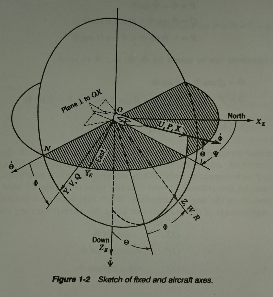
Figure 1-2 near the end of the Blakelock Chapter 1 extract below offers a helpful illustration and legend describing the body frame, fixed NED frame, and Euler angles. Here’s the figure. See the PDF below for a detailed description on pages 15 and 16.

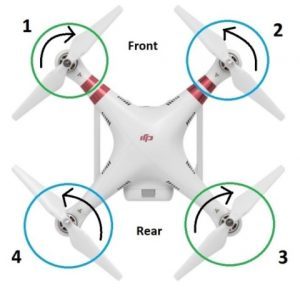
The sketch below illustrates a coordinate system fixed to the body of the quadcoptor. The X-Axis is defined to point always from the CG to the location of the first propeller. The Y-axis points towards what I label as the fourth propeller axis, and again by right-hand-rule Z is orthogonal to body X-Y plane by the right-hand-rule.

For now we make a design assumption that our quadcoptor will be a square cross configuration and not an, “X-wing” form-factor. There’s no particular reason other than wanting to sketch it this way and keep the diagrams and coordinate reference frames as simple as possible.

ref_frames

Angular Equations of Motion

The Bouabdallah paper refers to the Lagrangian method before summarizing the equations of motion for the 3 rotational axes as described above. I had some difficulty following the author’s use of Euler Angles and I’m not sure the derivations use these angles consistently within the paper.

Let’s try a Newton-Euler method (Morin p.376) because although the Lagrangian method is elegantly simple equating the rate-of-change of body momentum to applied forces and torques straightforward.

Recommended Reading

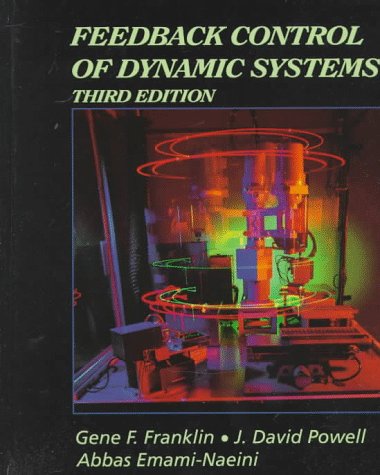
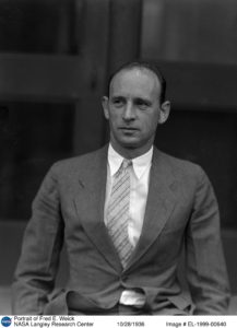
The following text as a, “classic”. The first edition was published in 1965, second edition in 1991. The first 10 pages of the first chapter lay-out the equations of motion for aircraft in a concise manner. Blakelock’s labeling and naming of the various body displacements, angles, rates-of-change of position and rotation, linear and rotational momentum, and his description of the Euler angles are helpful.

Retired USAF Colonel Blakelock died in 2015. Click his picture to read his obituary. I am thankful he left behind this great book for us.

It is confusing to think back-and-forth from the, “inertial” frame and the “body frame”. Specifically, the rotations on the body that an eventual gyro package will measure as (p,q,r) where…

p = Rotational rate of the body rolling about the body X-axis.

q = Rotational rate of the body pitching about the body Y-axis.

r = Rotational rate of the body yawing (twisting) about the body Z-axis

Then there are, “Euler Angles” (\Phi , \Theta , \Psi )  representing roll, pitch, and yaw, respectively. These are relative to the fixed-frame: the local NED coordinate system in our case.

Blakelock’s first 10 pages offer a clean and clear description that we will later see gets us to the equations in our main reference for the quadcoptor: the Bouabdallah paper.

Blakelock’s straightforward equations-of-motion derivation is included here:

blakelock_eom2

Timeout: Angular Momentum Clarification

In a linear system we know the simple statement, “momentum equals mass times velocity”. We know that linear motion in three dimensions means that velocity is a vector with x-, y-, and z-components. Mass for linear momentum is lumped to a point (our ball-bearing example above). It is a scalar. So, in a linear system we’re left with a momentum vector: the mass times the 3 components of it’s velocity.

A rotational system in three-dimensions will have a rotational momentum vector as well, but in this system, “mass” is represented as, “moment of inertia (I)” and velocity is angular velocity of the entire body represented as a three-coordinate vector \omega or \Omega  (capital or lowercase may vary but it is almost always this Greek letter, “omega”that is used).

At any instant you can think of this \omega-vector as the axle on which the body spins.

To complicate matters further, what was a scalar mass for the linear system becomes not simply a vector of inertia about various axes but a 3×3 matrix!

we’re going to ultimately arrive at a 3-element vector of angular momentum when we multiply our, ‘I’ matrix by our body angular velocity vector \vec\omega .

\vec L\:=\:\b I\vec\omega

First let’s get more comfortable with the inertia matrix, ‘I’.

Platform Inertia Matrix

The Blakelock text above skips over the details of the, “Inertia Tensor”: a matrix that represents the moment of inertia of the body. These are the, “I” terms. Good treatment of this topic is provided by David Morin in Ch. 9 of, “Classical Mechanics with Problems and solutions“. This Chapter is extracted here for your reference. The matrix describing a body’s moment of inertia is covered beginning on P. 376.

MorinCh9

Angular Momentum Changes

Page 393 in Morin above states, “Angular momentum, ‘L’ in the body frame changes relative to the fixed-frame (our NED frame) by two effects”..

  1. Body coordinates change relative to the body frame.
  2. The body frame itself rotates with respect to the fixed-frame.

Morin sets \vec L_0 = \vec L  as the momentum vector of the body at any given instant and imagines painting it on the body at this instant. The rate-of-change of momentum with respect to the fixed-frame is then…

\frac{d\vec L}{dt} = \frac{d(\vec L- \vec L_0)}{dt} + \frac{d\vec L_0}{dt}

That first term is the rate-of-change of momentum with-respect-to the body frame. This is what someone sitting on the rigid body would measure:

\frac{\delta \vec L}{\delta t} = \frac{d(\vec L- \vec L_0)}{dt}

The remaining \frac{dL_0}{dt}  term is the rate-of-change of the body-fixed momentum vector which is the body momentum at this instant as defined above. The momentum vector in this instant is assumed, “painted” on the body like our body axes. This temporarily, “constant” momentum is rotating with respect to the fixed NED frame on the ground at this instant. This is the \frac{dL_0}{dt}  term.

Morin reminds us that the fancy sum above that gives us total change in momentum \frac{d\vec L}{dt} is saying just this:

The total rate-of-change of angular momentum is the rate-of-change of momentum relative to the moving frame PLUS the rate-of-change of the momentum of the moving frame with respect to the fixed frame.

When we have any number of, “reference frames” for vectors this is how we map any vector from one frame to another. There is nothing magic or new here, even though the nomenclature looks fancy.

Body-Fixed Momentum Vector Relative to NED Frame

Just as Blakelock on page 13, Morin p. 93 gives us,

\frac{d\vec L_0}{dt} = \vec\omega \times \vec L

In Morin chapter 9 you can see derivation of the, “Inertia tensor” but it simplifies to a diagonal matrix when we select the body-frame axis to be principal axes of the body.

I =\begin{bmatrix} I_x & 0 & 0\\ 0 & I_y & 0\\ 0 & 0 & I_z \end{bmatrix}

Blakelock doesn’t zero the lower-left and upper-right terms of the inertial matrix. For a fixed-wing aircraft he maintains a cross-coupling of the inertia terms associated with roll and yaw. If you study his figure 1-2 in the book section above you can make sense of this for an aircraft that does not appear symmetrical front-to-back. However, our quadcoptor is symmetrical here too. Our inertia matrix simplifies to the diagonal matrix above.

This leaves us with L_i = I_iw_i for each body axis x, y, and z. The cross-product  \vec\omega \times \vec L  can be computed via the determinant of the matrix below. The determinant of a 3-by-3 matrix can be had by augmenting it with the first two columns as shown and subtracting left-diagonal products from right-diagonal products.

\begin{vmatrix} \hat x & \hat y & \hat z\\ w_x & w_y & w_z\\ I_xw_x & I_yw_y & I_zw_z \end{vmatrix} \begin{matrix} \hat x &\hat y \\ w_x &w_y \\ I_xw_x & I_yw_y \end{matrix}

Below are the hand calculations for the  \vec\omega \times \vec L  cross-product. The black lines represent the, “right diagonal” products. the red lines represent the left-diagonal products.

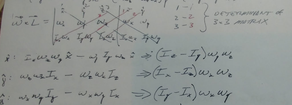
These hand calculations agree with Blakelock equations 1-32 (the central term with the principal axes moments of inertia in parenthesis). Our rotational rates match Blakelock’s as follows:

\omega_x = P \\ \omega_y = Q \\ \omega_z = R

These are the body rates-of-rotation about the principal axes of the body: the frame, “painted” on the body. We will soon get into details for an Inertial measurement unit (IMU) with gyros that will give us (p,q,r) data for our attitude controller.

Rate-of-change of body momentum relative to the body frame: \frac{\delta \vec L}{\delta t}

This is what we would measure if we were sitting still on the body.

As in Blakelock’s equation 1-32 we will assume the primary-axis inertia terms are constant. For aircraft, missiles, and the like fuel burn changes mass and distribution of this mass within the body. Our battery-powered quad will not experience these changes, but it worthwhile to consider this effect should we desire to deliver a payload with our quadrotor. When we drop the load the mass and moments would change.

Blakelock indicates that even when this is relevant for fuel-thirsty aircraft the above assumption works over time intervals much longer than our tens-of-Hz platform control loop. We would implement a, “sliding” controller or, “gain scheduling” system that effectively remodels our design periodically as fuel is consumed or payload is released. between those slower updates we would take our moment-of-intertia, “I” terms as constants.

Thus, we have

\frac{\delta \vec L}{\delta t} = (\dot PI_x, \: \dot QI_y,\:\dot RI_z)

Combining this with the result above our equations of rotational motion become…

\sum_{}^{} T_x = I_x\dot\omega_x\:+\:(I_z-Iy)\omega_y\omega_z \\\sum_{}^{} T_y = I_x\dot\omega_y\:+\:(I_x-Iz)\omega_x\omega_z \\\sum_{}^{} T_z = I_x\dot\omega_z\:+\:(I_y-Ix)\omega_x\omega_y

If you assume no applied Torques T (natural rotational response of the system) you can rearrange the above equations to match the Bouabdallah paper equation (6). Note that the, “I” subtractions are reversed because assuming zero applied torque we move terms to the other side of the equal sign and solve for the angular acceleration.

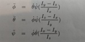
These match when we relate Bouabdallah’s terms to our terms above as follows…

\dot \phi = \omega_x \\ \dot \theta = \omega_y \\ \dot \psi = \omega_z \\ \ddot \phi = \dot \omega_x \\ \ddot \theta = \dot \omega_y \\ \ddot \psi = \dot \omega_z \\

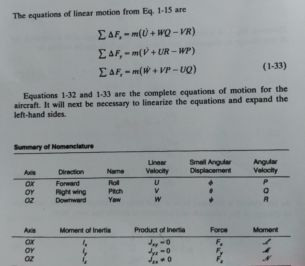
Equations of Linear Motion

The Bouabdallah paper describes a test-stand for which various various control strategies are studied. The test stand pins the CG to a point, constraining it to angular motion only. The paper does not cover details for linear motion.

Blakelock chapter 1 above offers good descriptions for modelling linear motion. Below is his conclusion. If you look back at his Equation 1.15 you can see how each primary axis velocity couples into acceleration of the other axes via another cross-product. I’m going to leave this here for now because depending on how we measure position and velocity relative to the body and/or fixed NED frame these terms may or may not be relevant in our design.


Conclusion

It looks like we have a good handle on the equations of motion now. We have nomenclature and methods for thinking within the two reference frames:

  • The North-East-Down (NED) frame pinned to the earth at our take-off point.
  • The Body frame we can think of as permanently painted along primary (x, y, z) axes of our quadcopter.

We’ll pick up the applied torque and force elements of the equations-of-motion in the next post. These are the following terms in the equations above.

\sum_{}^{} T_{(x,y,z)}\\ \sum_{}^{} F_{(x,y,z)}\:

They are the torques and forces that will act on the quadcoptor. They will include the desired outputs from the propulsion units, and we can also model external factors such as wind. We will need a controller design that is robust to some applied, “disturbances” from wind.


Quadrotor Dynamic Model: Propeller Gyroscopic Effect.

The equations below are from the last post, where we see we matched our Bouabdallah paper‘s equations for rotational motion.

We know some propeller input is going to be a part of the applied torque. There is going to be a set of equations for linear motion too, but let’s clarify what is going on here regarding torques about our 3 body axes. Let’s look at these equations and…

Review Rigid body rotation gyroscopic effect

\sum_{}^{} T_x = I_x\dot\omega_x\:+\:(I_z-Iy)\omega_y\omega_z \\\sum_{}^{} T_y = I_x\dot\omega_y\:+\:(I_x-Iz)\omega_x\omega_z \\\sum_{}^{} T_z = I_x\dot\omega_z\:+\:(I_y-Ix)\omega_x\omega_y

Remember Newton’s Second Law \sum F_i=m\cdot a_i? This tells us that the sum of the forces on a mass in the i’th direction must equal the mass of the body times the acceleration in that direction.

If we take one of the equations above and rewrite it we can recognize this familiar form, albeit in rotational nomenclature. The rightmost term is the gyroscopic effect of the entire rigid body. It tells us that if there is rotational rate about y- and z-axes a torque is induced about the X-axis. If we neglect this term you see we’d be left with  \sum_{}^{} T_x = I_x\dot\omega_x in simple second-law form.

It’s a little confusing, but all we’ve done is already offer one item to the, “sum-of-torques”: the gyroscopic effect resulting from the rigid body rotation. Notice when we moved the term in parenthesis to the other side it looks like an added torque now but we swapped the subtraction in parenthesis so the math is the same.

I_x\dot\omega_x = \sum_{}^{} T_x \:+\:(I_y-I_z)\omega_y\omega_z

Gyroscopic effect of Propellers rotation.

“tail-dragger” airplane example

The video below to describes a phenomenon familiar to pilots, particularly pilots of powerful, “tail draggers” like the P-51 Mustang. A propeller is a large spinning disk. When we tip the plane of rotation of the propeller: pitch the airplane, a torque on the body results due to this gyroscopic effect.

Imagine you are in the cockpit of the P-51, speeding down the runway (lucky you). That monster prop has a healthy angular momentum vector pointing perpendicular to the prop. Your tail is dragging until you get enough lift from your wings (due to streamline curvature, if you recall a recent post!). At some point your tail will lift and you’ll be parallel to the ground before your front wheels leave the ground. This looks like a quick, “pitch” of say 15-degrees based on the photo above. Let’s say it took a second for the tail to rise as we’re nearing take-off, so the pitch rate is 15-degrees per-second as the tail wheel leaves the ground.

That same pitch is pitching the plane of the spinning propeller forward, or more to the vertical. When you watch the video below and inspect the equations below you will see that this, “pitch forward” of the propeller at the above angular rate of the airplane going from dragging-to-level results in a gyroscopic torque about the airplane’s vertical axis: you feel the plane want to yaw (twist) so you’ll need to correct with some rudder.

The effect can be negligible

Our propellers are horizontal in the body-plane, but there is a torque induced on the body that results from propeller rotation and rotation of the propeller plane about the x- and y-axis of our system too…at least in theory. It may be negligible depending on propeller moment of inertia relative to other effects, but let’s model it anyway.

We can choose to include it or neglect it later when we perform a sensitivity analysis. This is where we can look at rough magnitude of various effects and decide to include them in our model or cancel the terms in the equations: ignore them as too small to make a difference. We’ll do this systematically and not guess at this point. Besides, this is a neat phenomenon for us to appreciate in detail.

Video Explaining Equation Derivation

Gyroscopic effect of our propellers

The following PDF derivations arrive at the same terms as the Bouabdallah paper (equation 8). There’s a sign convention difference between the paper and these derivations, but the result is the same:

T_{x,prop}\:=\:I_{prop}\cdot\dot{\phi}(\omega_2+\omega_4-\omega_1-\omega_3)\\ T_{y,prop}\:=\:I_{prop}\cdot\dot{\theta}(\omega_1+\omega_3-\omega_2-\omega_4)

The first equation tells us that there will be a torque about our body X-axis when there is angular rate-of-change to our pitch: \dot \phi (not the dot, implying pitch rate). This means our quadcopter will feel a  body roll-inducing torque when it pitches. This is due to the gyroscopic effects of the 4 propellers.

The second equation tells us that there will be a torque about our body Y-axis when there is angular rate-of-change to our roll: \dot \theta. This means our quadcopter will feel a  body pitch-inducing torque when it rolls.  Again, this is due to the gyroscopic effects of the 4 propellers.

The hand calculations below arrive at the above equations following the process in the video. The video above explains how to go about the hand calculations for a single propeller.

Hand Calculation PDF Notes

RB 2018-07-11 17.27.01

Conclusion

If you expand these equations you’ll see I just performed the steps in the above video Eight times and combined the equations. We need eight steps because we have 4 propellers and we need to account for the plane-of-rotation rate-of-change about both the x- and y-axis. Rotation about the body z-axis contributes no gyroscopic effect from the propellers because it is just like twisting the axis of the propeller. The plane-of-rotation of the propeller does not change in this case so no torque is induced on the body.

T_{x,prop}\:=\:I_{prop}\cdot\dot{\phi}(\omega_2+\omega_4-\omega_1-\omega_3)\\ T_{y,prop}\:=\:I_{prop}\cdot\dot{\theta}(\omega_1+\omega_3-\omega_2-\omega_4)

We’ve now accounted for gyroscopic effect of the rigid body rotations and the propeller rotations.

Next we’ll add the propeller thrust components. These will be our inputs to counteract the above effects and unknown disturbances (wind) in order to maintain the attitude of our quadcoptor and move it where we want it to go.