Motor-Prop Model Validation
[latexpage]
In a recent post we used the Tyto 1520 test stand to get at a maximum thrust available from our motor-prop system. We want that maximum thrust so we can normalize our LQ controller command output for the Ardupilot motor command as outlined here. The Tyto 1520 offers great value for under \$200.
While we have it set-up, let’s also have some fun validating our motor-prop equation and parameters!
Review Motor-Prop Mathematical Model
Modelling the motor-prop assembly is where the quadcopter deep-dive started way back here. Since that time we took some time to appreciate propeller fluid mechanics, and drag and thrust coefficients. We started with this…
$\frac{d\omega}{dt} = A\omega + Bu +C$
Where…
$A = -(\frac{K_m^2}{RJ} + \frac{2d\omega_0}{\eta r^3J})$
$B=\frac{K_m}{RJ}$
$C = \frac{d\omega_0^2}{\eta r^3J}$
But as rationalized here we eliminated the, ‘C’ term and adjusted the A term accordingly to arrive at…
$\frac{d\omega}{dt} = -(\frac{K_m^2}{RJ} + \frac{d\omega_0}{\eta r^3J})\omega + \frac{K_m}{RJ} V$
Where, ‘V’ is DC voltage. By inspection we see this equation tells us that on the moment we apply a voltage, ‘V’ the term multiplying it is all about the motor-prop ability to spin-up while the negative term preceding on omega enforces the drag.
Another way to think about it is to observe that at some steady-state for a constant voltage input, ‘V’ if we remove V that second term becomes zero and the first term conveys spin-down of the system due to mechanical and electrical effects.
Comparing the step-response of our model using Matlab to data we collect on our test stand permits us to check some parameter assumptions to this point.
Test Stand Step Response
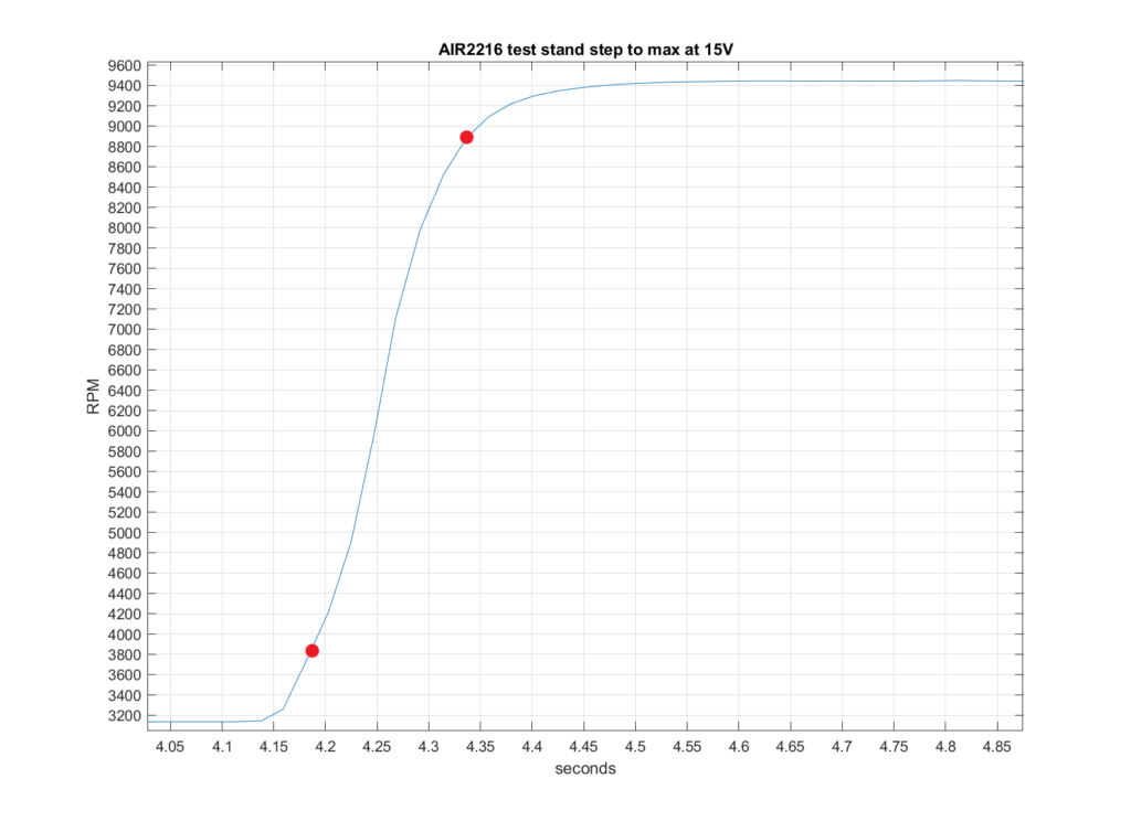
The Tyto RCbenchmark software permits scripting a step sequence to maximum output. The test stand is set-up to step from zero to 20%, hold, then step to 100% output. This step from spinning at 20% to maximum is our reference for model validation.
The red dots below represent the step from 10% to 90% RPM output on the transient from 20% spinning start to 100% from the electronic speed controller (ESC). This indicates a step response of 4.33-4.18= 150ms. We don’t step the prop from a dead-stop.
The start-up motor dynamics are too messy to contend with. Think of it like not wanting to model, “stiction” or what it takes to get something sliding. We want to make a step-change once sliding and avoid all the unknowns from zero. Hence we start our test stand from 20% output on the electronic speed controller, which produces near 3200RPM.
We’ll start our simulator from the same 3200 RPM too, although it doesn’t suffer from a zero start because it’s an ideal, first-order model, albeit with modelled nonlinearity in omega.
Steady State Comparison
The first thing we want to do is check our parameters at steady-state
- Set V to max test voltage = 13.85 V
- This is the Maximum at steady-state with voltage droop from 15V on our test stand so…
- Use this for steady-state model voltage
- Steady-state so…
\begin{equation} \omega_0 = \omega \end{equation}
\begin{equation} \frac{d\omega}{dt} = 0 = -(\frac{K_m^2}{RJ} + \frac{d\omega}{\eta r^3J})\omega + \frac{K_m}{RJ} V \end{equation}
Rearranging…
\begin{equation} \frac{K_m^2}{RJ}\omega^2 + \frac{d\omega}{\eta r^3J}\omega – \frac{K_m}{RJ} V = 0\end{equation}
Quadratic equation to solve for omega…
\begin{equation} \omega = \frac{-K_m^2+\sqrt{K_m^4+4RdKV}}{2Rd}\end{equation}
Our largest uncertainty is likely the, ‘d’ term: the drag coefficient for our propeller. Motor resistance, ‘R’ is another uncertainty, while motor constant Km is had from 1/Kv where Kv equals the advertised 880 RPM/Volt.
Estimate Drag Factor From Test Stand Data
We measured max 9500 RPM (~1000 rad/s) above at Vmax=13.85 so to solve the above equation for our most uncertain parameter pair R and d.
- ω = 1000 rad/s
- V = 13.85
- Km = 1/Kv = 1/880 RPM/volt = 0.011 (converting to radians and seconds)
Rearrange the Quadratic equation and solve for Rd…
Rd = 3.135 x 10⁻⁸
where
\begin{equation} d = \frac{P_{const} \rho D^5}{8\pi^3} \end{equation}
If we take motor resistance as 0.115 ohms our test stand estimate for drag factor, ‘d’ is…
d = 2.73 x 10⁻⁷
Model Drag Factor
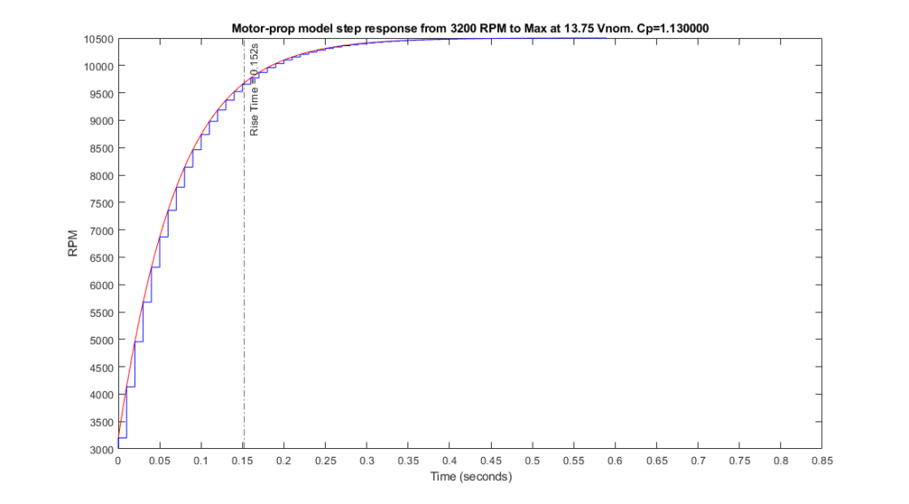
The model gives d=1.5 x 10⁻⁷ when we accept the Ardupilot SITL script assumption for propeller power coefficient Cp=1.13. Both model and above operation on test stand data assume same value for motor coil resistance of 0.115 Ohms.
For Cp=1.13 the model also produces a higher steady-state result. observing the figure below
Model Parameter Adjustment
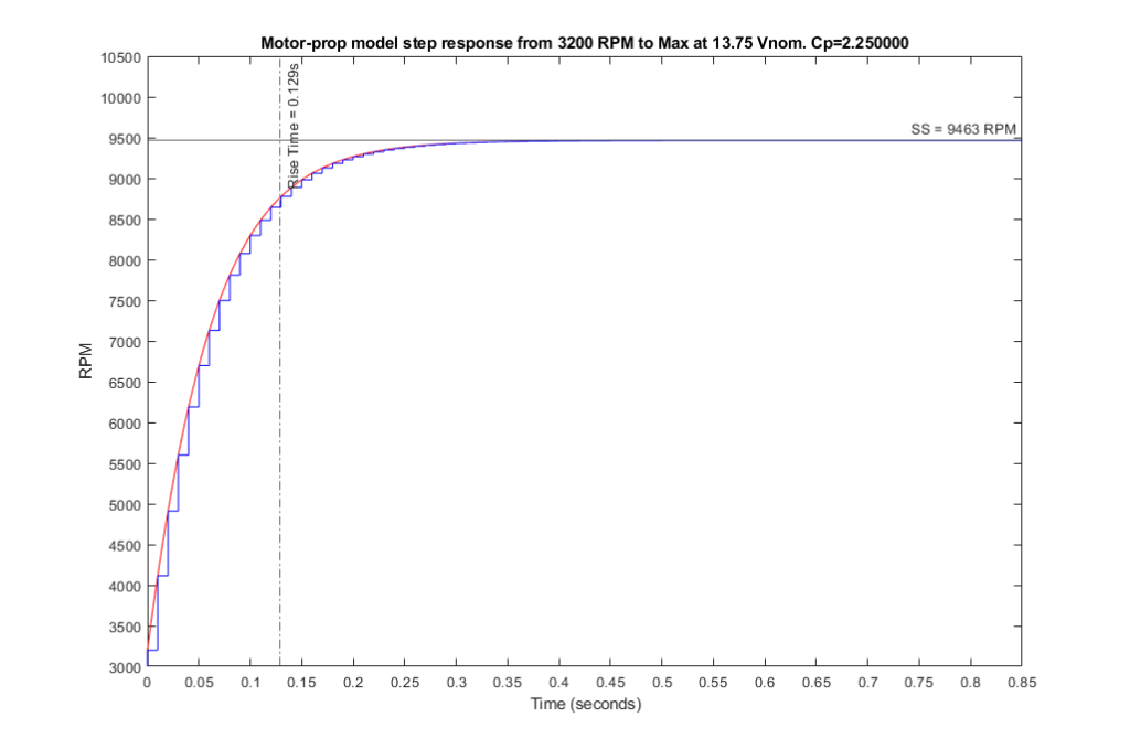
Changing the model power coefficient to Cp=2.25 yields a steady-state RPM in-line with the test stand result and a rise time that is still within 15% of the measured rise time (129ms below compared to 150 above). The test stand output plot indicates some higher-order response from zero. We don’t have those dynamics modeled. Given we have some unmodeled higher-order 129/150= 86% match on rise-time with match on steady-state is close.
Let’s conclude that our SITL Cp is too low at 1.13, and that Cp=2.25 is closer to actual than 1.13.
With model Cp=2.25 the model’s drag coefficient d = 2.97 x 10⁻⁷, within 10% of our estimate of d = 2.73 x 10⁻⁷ for the test stand.
Conclusion
Motor-propeller power coefficient (Cp) taken as 1.13 from the Ardupilot SITL (simulator in-the-loop) appears low. Increaing model Cp to 2.25 produces a close match on steady-state output between test stand and model for a modelled-as-same voltage step input.
Cp=2.25 yields a rise-time estimate 15% faster than the test stand. However, considering the higher-order response from intitial RPM for the test stand that we don’t have modelled this appears reasonable when examining the plots above. If the model rise from zero were higher-order like the test stand reveals this would increase the first-order simulated rise time of 129ms above, closer to the measured 150, closing the 15% error to some degree.
With Cp=2.25, a close match on steady-state output and a model simulation rise-time within 15% of measured, given our somewhat crude tools and basic methods here, let’s call the model, “validated”!