Quadrotor Linear Quadratic Regulator (LQR)13 min read

October 10, 2020

Big gap since the last post where we finally got the state-space model laid down. It got us to the plant model derived by Bouabdallah and others in his paper that we’ve used as a guide from the start.

The goal all along has been not only to analyze and design candidate controllers for a Quadrotor platform, but to take forays into applied math, mechanics, and advanced techniques that we might not need for a camera hover drone but which give us a chance to stretch our skills.

A typical quadrotor controller decouples the roll, pitch, and yaw axes and implements PID controllers for each axis as described in our post from awhile back. We know this works, and we could jump into Ardupilot source code for say a PixHawk Cube and see exactly where and how PID controllers are implemented in source code.

Instead of getting into an implementation let’s push on to learning Linear Quadratic control techniques for a Multi-Input, Multi-Output (MIMO) system.

Why State-Space Model and LQ Control?

The axis decoupling created Single-Input, Single-output (SISO) systems out of the Roll, Pitch, and Yaw axes and expects each axis to work independent of the other via PID control, or more specifically via a lead compensator as illustrated earlier. This is an adequate, in most cases a good, robust design so why am I making this more complicated? It might be bad engineering practice for a simple camera drone, but as we are not designing a specific drone just yet, we’re keeping some extra terms in our design. We’re working on the general case still: a wide flight envelope away from small-signal hover response.

Retain Inertial Effects: Axis Coupling

We’re keeping body inertial effects and propeller gyroscopic effects in the model. These null-out for roll-, pitch- and yaw-rates near zero, at which point the state-space A and B matrices simplify to what are basically 3 independent axes of control, a situation where our Lead compensator applies. By not assuming these terms negligible we retain cross-axis coupling and can’t treat the platform as a set of three independent axes controlled separately from one another.

Comparisons with Classical Approach

The classical design method is a bit more intuitive compared to an LQ optimal approach where we pick relative weights for state convergence cost and control cost (more on this later). Recall the insight we gained about plant dynamics and dominant poles that limit plant response: body and prop moments of inertia. This is intuitively obvious: large, heavy rig and slow prop response limits ability to accelerate body rotations. We could see these factors in Bode plots and scale our crossover accordingly. The math and our intuition were well aligned.

When we compute a linear quadratic gain matrix we’ll be pumping our intent through the calculus of variations and some formulae that seem like magic. We’ll compute, “optimal” gains according to a cost function. We’ll gain some insight by varying our design parameters but it will be an iterative process relying on comparative analysis of simulations. It won’t be as prescriptive as frequency design methods or pole placement in general.

Also, “optimal” is a bit of a misnomer. An, “optimal” gain is only so relative to a particular combination of state and control weights. It’s not, “optimal” in an engineering sense, only in a mathematical sense for the weighting parameters we supply.

Starting Point: Full-State Feedback Regulator

We’ll eventually add roll, pitch, and yaw reference inputs that a flight controller outer loop will command. These will be the reference inputs to this inner platform attitude control loop that we are familiar with from our classical control designs. However, to get started let’s implement a simple full-state feedback regulator. This will get our design and simulation tools in order before we introduce reference inputs.

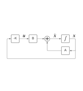
Below is the system model: full-state feedback to gain K with state transition matrix A, and input matrix B. Another simplification here is the availability of state measurements for feedback. We can expect to have measurements from gyros and accelerometers but these will feed a state estimator that will in-turn supply the full-state feedback in our loop. However, state estimation is another topic, and it can be decoupled from the controller design. We’ll cover it later.

When we ultimately add reference inputs and state estimation to this diagram it will represent a design for implementation, but in diagram form it will look more intimidating than this picture. Let’s learn from this first, and build on it.

Full-State Feedback Regulator Block Diagram

State Definition

Our state vector, ‘x’ contains roll, roll rate, pitch, pitch rate, yaw, and yaw rate, respectively:

x=[\phi\;\dot{\phi}\; \theta \;\dot{\theta}\;\psi \;\dot{\psi}]^T

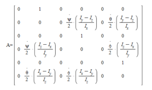
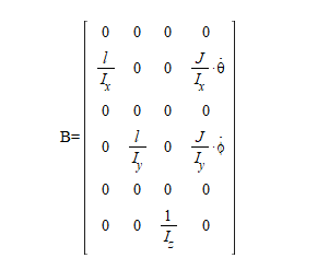
State Transition Matrix A and Command Matrix B

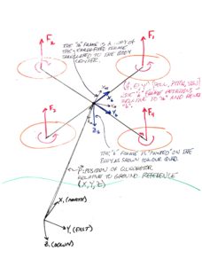
Quadcopter Body Model Sketch

Feedback Gain ‘K’

This is will be an optimal control solution. In this post we will rely on Matlab’s LQR() function. You’ll see the call in the Matlab script later but first,

There are States in the Transition and Control Matrices, Why?

As we recall from the last post and can see above, the A and B matrices have the three rate states within. Had we not employed Bouabdallah’s trick to add the rates as states themselves we’d have a product of rates in elements of A. We eliminated this non-linearity, but we still have states in A. This is not invariant throughout flight.

Options for dynamic flight when body and prop dynamics factor-in to A and B..

Model small-signal near-hover control: zero the rate states in the A matrix
1. This is basically what we did for the classical design methods. It permits decoupling the axes, at which point this LQR method is less intuitive that 3 decoupled control loops designed as described previously
Recalculate Control Law K over the flight envelope: successive linearization.
1. To the furthest extent this involves taking output rate states as inputs to A and B which are then inputs to a solution of the Matrix Ricatti equation resulting in gain matrix K.

Given we’ve already pursued Step #1 in our classical design approach, let’s push ahead with approach #2

Successive Linearization of the Plant Model: A and B Matrices

It would be impractical to recompute feedback gain K as a function of revised A and B matrices for each new sample (estimate) for $[\dot{\phi}\;\dot{\theta}\;\dot{\psi}]$ in our control loop calculations. Our platform control loop would be solving the matrix Ricatti equation in real-time.

A practical design could be a three-index look-up table that covers the range of these body axis rotational rates with a reasonably granular step size. This look-up table could contain pre-computed gain matrix K corresponding to the lookup value indexed by current $[\dot{\phi}\;\dot{\theta}\;\dot{\psi}]$ . Let’s assume something along these lines as a design direction later.

For the simulation that follows we employ Matlab’s LQR function in a loop and we successively compute control gain matrix K. This allows us to visualize the regulator process using the power of the simulation tools before adding complications: reference inputs, gain scheduling from look-up table, and other practical details.

The Control Law: Computing K

Our objective in this exercise is to regulate to zero state-vector X governed by differential equation

To minimize performance measure

J=\frac{1}{2}\int_{t_{0}}^{t_{f}} \left [ x^{T}(t)\;Q\;x^{T}(t)\:+\:u^{T}\;R\;u^{T} \right ]dt

The performance measure employs two matrices Q and R to weight the importance of state convergence and control effort, respectively. Derivation of the performance measure and how the plant differential equation and this performance measure combine to determine an, “optimal” controller gain K given A, B, Q, and R is a topic for a lengthy foray into optimal control theory and the calculus of variations.

We’re going to skip this for now and simply use Matlabs lqr() implementation to meet the stated objective and supply us with a gain matrix K. By first visualizing through simulations what we are achieving with these methods we’ll have perhaps a greater appreciation for the details when we dive into all the math behind Matlab’s “lqr()” function.

We will see the relative effects of Q and R on regulator performance. We’ll then move on to the tracking problem when we are not regulating states to zero, but attempting to track reference inputs for these states. An outer flight control loop will supply these references for tracking targets in flight, for example.

For now let’s accept the performance measure as a result of something called the, “second variation” in the calculus of variations, employed for neighboring-optimal solutions. The final time in our definite integral is also, “free” but we’ll cover that later

Regulator Simulation

This basic regulator simulation is the foundation for complexities we’ll add as we go: tracking reference inputs, state estimation, and introduction of actuator limits, plant uncertainties, and disturbances.

For now we want to get the simulation correct by observing ideal condition regulation to zero from initial conditions on roll, pitch, and yaw. The video below represents simulation output from the Matlab script explained below.

Method

The plant is modelled in continuous time. An outer simulation loop is equivalent to sampling time of a physical system: the interval on which states would be sensed and/or estimated and updated commands actuated on an actual system.

In the simulation the system is the plant model A and B as coefficients of the state differential equations. On each iteration of the sampling loop the time interval is further divided into time steps over which Matlab’s ode45 integrates the state differential equations.

Each invocation of ode45 takes as initial conditions for the states the last state output from the last invocation. Ode45 solves the system below on each invocation for a time vector that represents the sampling time interval further divided, computing a state estimate x for each step of that finer interval.

Command input, ‘u’ is constant for each invocation. It represents operating on feedback from the previous loop, applying the controller gain K, and issuing an update command, ‘u’ to the plant.

function xd = ssodefunc(t,x,a,b,c,u)
xd = a*x + b*u;
end

After each invocation the full simulation time vector is appended with the new timesteps from ‘t’ and the state estimates are appended to the full simulation state estimates.

Think of it as though we are kicking a continuous (analog) system on a time interval with updated commands, ‘u’. The analog nature of the plant is represented by the finer time steps for which Ode45 produces state estimates. All of these between-sampling-interval state estimates represent the actual motion of a physical system.

By taking the last Ode45 state solutions from each interval as initial conditions for which to use as feedback to control gain K and as initial conditions for the next iteration we are simulating as though we are, “sampling” (with sensors) on this interval, as if we only know the last solution from each invocation of Ode45.

By plotting every finer interval it is as though we are observing the behavior of the continuous-time, analog system under the control of our sampling-and-control system.

Simulation Details

The Matlab M-file below implements the simulation described above. I use a, “home use” license of MATLAB R2019b with the Control Systems toolbox and the Signal Processing toolbox although you likely need only the former. Mathworks, “home use” licensing is a great recent offer. For a couple hundred dollars you can add this to your tool set. In the past I benefitted from commercial licenses I had access to for work. It’s great to have a personal license. I highly recommend it.

Matlab Script

The plant parameter values are as derived in an earlier post where we implemented the classical lead compensators for roll, pitch, and yaw.

“tstep” is our control loop sampling interval. It has a basis in the reality of our band-limited mechanical plant. Recall we closed the classical loops with unity gain crossover at 10Hz. If we imagine tracking a disturbance in this range, how fast do we need to sample? I remember some old design rules of 5 or greater times sampling frequency relative to loop crossover, so this implies we want to be in the neighborhood of 50-100Hz sampling frequency. This sounds about right.

If you play with this simulation with slow tsteps of ~0.1+ seconds you’ll see the system go unstable. This is because we’re sampling the plant too slow relative to the inherent dynamics. On the fast side we would run into computational and sensor limits, but it’s reasonable to assume a 50-100Hz sampling rate for this platform control loop will be achievable in hardware.

Below you will see tstep=0.02s representing a 50Hz control loop. Imagine this would be the rate at which we would sample sensors, update state estimates, and issue revised commands to our motors. This might be a bit slow but it’s fine for now. 50-100Hz is likely what a hardware platform will support. There will be other sampling rates within the system to, for example, acquire inertial sensor data and filter estimates for the platform control loop. These may run considerably faster, and we will, “sample” the output of these subsystems for estimated at our control loop sampling rate.

Download the M-file

three additional supporting functions to place in same folder when you run the above script: paintbody.m, paintbody_update.m and ssodefunc.m

Conclusion

We introduced a simple multi-input, multi-output (MIMO) Linear Quadratic Regulator design and simulation here with full-state feedback. State feedback will ultimately come from a state estimator: a Kalman filter that will perform sensor fusion from our gyroscopes, accelerometers, GNSS (GPS), compass, and barometric sensor on a real flight platform.

This state estimation will be a topic all it’s own. We’ll also later introduce reference inputs for pitch, roll, and yaw so we can control to setpoints and not simply regulate to zero values.

Until then, study and play with the m-file above if you can find yourself a Matlab seat!