Linear Quadratic Control with Reference Input

March 31, 2021

The last post was our introduction to the Linear Quadratic Regulator (LQR). We saw there that as we started with initial conditions or introduced a disturbance the LQR will drive the states to zero. In the simulations we saw the graphic of the copter converge on the zero state: zero roll, pitch, yaw, and respective rates all to zero.

The, “Control Law” (feedback gain K) was obtained through a solution of the matrix Ricatti equation buried in Matlab. We’ll dig into that math at some other time.

This same solution is relevant for the, “tracking” problem or servo case: when we desire the plant to be controlled to a particular set of non-zero state values.

Table of Contents

Basic Idea

We can think of it as the reverse of our last simulated cases where we started with non-zero state initial conditions (some angles for roll, pitch, and yaw) and observed the platform converge on the zero-state attitude.

Think of this new problem as starting with zero initial conditions (a level quadcopter) and desiring the attitude, “step response” to a non-zero input.

This is a bit artificial for the quadcopter because a non-zero attitude will mean thrust in a particular lateral direction which we are ignoring at present. Our controller design will still be relevant, as this is the attitude control loop.

Ultimate Goal

Later we’ll introduce an outer position control loop that supplies the reference inputs to the attitude controller: the reference input that is the topic here. In flight it will not be a set value but a continually changing attitude reference input based on the outer position control loop’s desire to move the platform by altering the attitude and the resultant thrust vector.

Before we can illustrate how an outer position controller will command attitude to this inner attitude controller we need to understand how to introduce the reference for roll, pitch, and yaw.

The respective rates are states also, but our goal is to regulate these to zero as the attitude tracks the body angle input reference. Our reference vector will supply zero for the rate states.

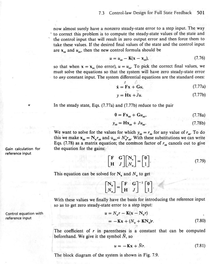
Theory

Feedback Control of Dynamic Systems by Franklin, Paul, and Emami-Naeini introduces the topic via the material below. The following page copies are from a 1994 edition of their textbook.

Quadrotor Implementation

We are dealing with more states and a multi-input, multi-output (MIMO) problem. The equation to solve from the reference above is shown here with bold matrix elements representing matrices themselves.

Our ‘A‘ and ‘C‘ Matrices are 6×6. The ‘B‘ and ‘D‘ Matrices are 6×4. This results in the matrix needing an inverse being 12×10, which is non-invertible. On page 510 Stengel writes we can employ the right pseudoinverse in this case.

(1) $\begin{equation*} \begin{bmatrix} \mathbf{N_{x}} \\ \mathbf{N_{u}} \\ \end{bmatrix} = \begin{bmatrix} \mathbf{A} & \mathbf{B} \\ \mathbf{C} & \mathbf{D} \\ \end{bmatrix}^{-1} \begin{bmatrix} \mathbf{0} \\ \mathbf{1} \\ \end{bmatrix} \end{equation*}$

We can then solve for the reference gains. The resulting N_x is 6×6. The resulting N_u is 6×4. We now have the matrices we need to operate on our state reference.

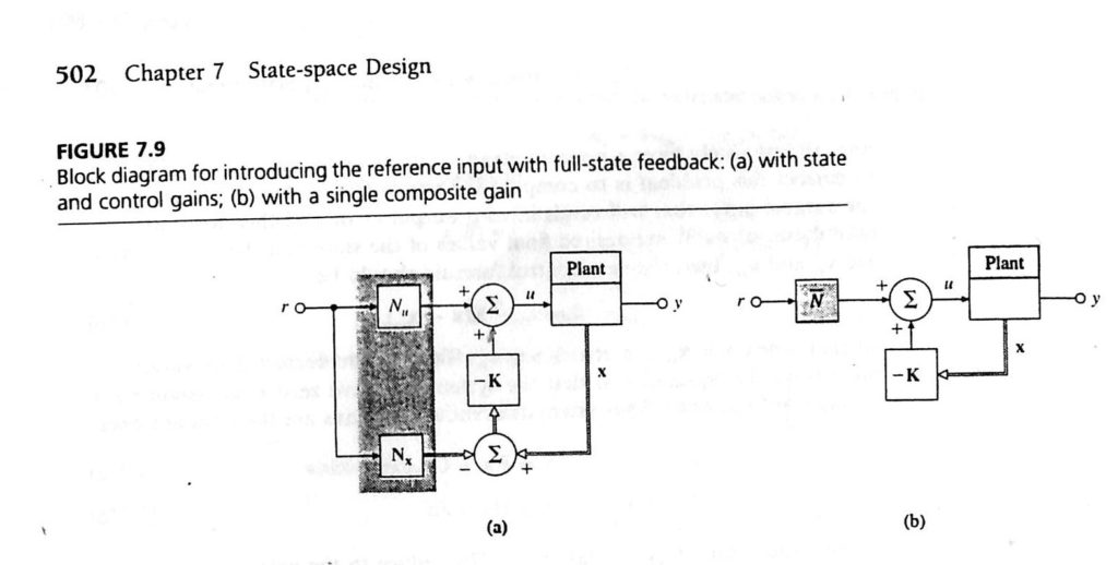
N_x and N_u are simplified into a composite gain in the second block diagram according to the reference textbook above:

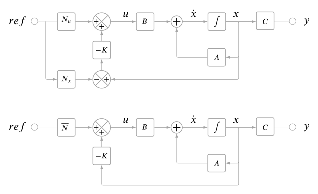
(2) $\begin{equation*} \bar{N}=N_u+KN_x \end{equation*}$

We’re now ready to see how the quadrotor LQ controller will track a reference input. The controller gain matrix K is from our LQR solution, so it’s the same controller.

Matlab Simulation

This Matlab script is a generalized version of the script in the last post covering the LQR simulation. In this script you will see the reference gain N is established and applied to a reference input. Yaw-axis sinusoidal reference tracking is illustrated in the following video generated by running the script.

You’ll need the same three additional files from the last post (see the matlab script section near the end).

Download the script, find yourself a Matlab seat, and explore!

Quadrotor Reference Input Tracking: a yaw-axis sinusoidal reference

Conclusion

We’ve covered how to solve for the reference input gain matrix and modified our LQR Matlab simulation script accordingly. The simple simulation shared in the video above indicates we’re stable and generally tracking the yaw sinusoid.

There’s more to do in this area: examine disturbance rejection, tracking performance, and general analysis of our LQR controller. Through this process we’d apply some performance assessment metrics and iteratively adjust our cost function weights.

We’re not yet to a real design and iteration process yet. We’re still building the tools and the understanding of how this MIMO Linear Quadratic quadcopter math works.

Happy Learning!