The last few posts covered each of three dynamic details separately:

Gyroscopic effect of the rigid body (the entire quadcopter).
Gyroscopic effect of the spinning propellers.
Propeller thrust and drag effects.

We’re going to use all of this information as we look at controlling the flight of a quadcopter, but first we’re going to make some simplifying assumptions so we can get to a, “classical” controller design around a transfer function.

After we attack the simple model we will try our hand at other techniques using state-space methods. Starting with a classical control loop model that neglects gyroscopic effects and cleanly separates the axes of control will provide a solid understanding of the physical problem. Then we’ll add-back the complications and try other design methods.

This first video walks through to the end result. See more detail below.

In the video I say, “theta” often when I should be saying, “phi”…it’s all Greek to me, as the saying goes.

Simplifications

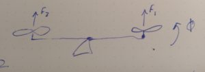
Let’s consider two propellers responsible for rolling the body, and pin the point of rotation at the balance point, as illustrated in the sketch here. both the roll and the pitch axis can be considered as such. We’ll cover yaw later. Here we are going to simplify the dynamic model in pursuit of a transfer function from propeller inputs (which produce thrust F1 and F2 in this sketch), and roll angle output $\phi$ . We need to make 3 simplifying assumptions to the model developed to this point, as described below.

1. Ignore Gyroscopic effect of the Rigid Body

Imagine the initial condition is a balanced one: we’re not amidst drastic changes to the level condition. We want to consider the response of the simplified model above to slight disturbances about the balanced condition. We might be relatively insensitive to the gyroscopic effect of the rigid body even under more dynamic conditions, but in any case this simplification allows us to ignore the rigid-body gyroscopic effect described here.

2. Ignore Gyroscopic effect of propellers

Again, if we’re hovering level we are not amidst rate-of-change of the rotational plane of the propellers, recalling an earlier post.

3. Neglect the, ‘C’ term in our propeller speed differential equation

The above simplification will get us to match the simplified model in the Bouabdallah paper, but I struggled to match the author’s reasoning for his final simplification: neglect the, ‘C’ term in the propeller speed equation (red highlights below).

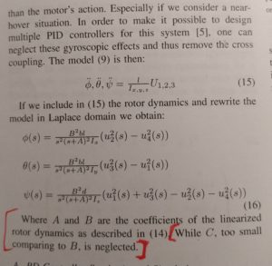
Challenged to validate, “C too small comparing to B”…

We need to plug some parameter values in for ‘B’ and ‘C’ to check Bouabdallah’s claim above. When we do so, the opposite is revealed: ‘C’ is greater than ‘B’!

The ‘C’ term is not small compared to ‘B’…we need it’s effect to be. How can we check this?

Simply comparing the magnitude of the B and C parameters for nominal conditions above doesn’t tell us if we can safely ignore B or C. We know we can’t ignore our ‘B’ term because this would zero our drive input! Se we’re stuck with what looks like a smaller value for B than C

Sensitivity Analysis: $\frac{d\omega}{dt}$ sensitivity to changes in ‘u’ and $\omega_o$

This video explains how to rationalize neglecting the, ‘C’ term and an additional adjustment to the ‘A’ term that results.

PDF of the document reviewed in the video justifying neglecting the ‘C’ term.

V_WSensitivity

Controller Drive Outputs

The Bouabdallah paper equation 10 simplifies the control inputs by combining the propeller inputs into intuitive combinations based on what we’ve derived so far. My sign convention is different with z-down in my case, but I’m following the lead of this paper to state the control inputs as…

U_1=b(\Omega _2^2 - \Omega _4^2)\\ U_2=b(\Omega _1^2 - \Omega _3^2)\\ U_3=d(\Omega _2^2 + \Omega _4^2-\Omega _1^2 - \Omega _3^2)\\ W =(\Omega _2 + \Omega _4-\Omega _1 - \Omega _3)

You can interpret the above as…

U₁= Roll input
U₂= Pitch input
U₃= Yaw Input

W = Propeller gyroscopic effect as a disturbance, “input”. We are ignoring this, for now.

The control logic is going to request roll, pitch, and yaw output from the platform as a combination of propeller drive inputs as above.

Resulting Transfer Function

After accepting the above simplifications and control input definitions we arrive at a transfer function from motor drive voltage (the difference of the squared drive voltages denoted capital ‘V’) and roll output. For a symmetrical quadcopter this transfer function applies the the pitch axis as well. We’ll cover yaw later (it’s just a bit different).

\frac{\phi(s)}{V(s)}=\frac{K_g}{s^2(s+A)^2}

With plant gain

The intro video up top and the following PDF cover the derivation of the final transfer function after accepting the simplifications above.

PDF from the notes reviewed in the intro video

simple_model

Conclusion

This post required more than I expected to rationalize ignoring the, ‘C’ term in the propeller speed equation! I’m glad to have wrestled with it, because my resulting adjustment to the ‘A’ term now appears more realistic than the expression in my reference paper.

Getting comfortable with simplifications to the propeller speed differential equation was the biggest leap required to simplify our model. Now we have a transfer function we can design a controller around. We will dig into this next time!

Quadrotor: Simplifications for, “Classical” Controller Design