Revisit the Motor-Propeller Model8 min read
It’s been fun to mess with the motor-propeller differential equation and linearization in an post. However, when I got into looking-up some rough parameter estimates and performing dimensional analysis (seeing if the units worked-out right for me in the equations) I ran into some problems.
I realized I was not only needing numbers, but I wasn’t comfortable with the units either! This means no controller design until we get a better understanding of the, “plant” (the thing we want to control: the propeller speed via the motor and gearbox if any).
Table of Contents
Backup and learn more…
The picture for this post shows a Mr. Fred Ernest Weick (1899-1993). I learned of him as I dug into some details relating to this post. I got stuck trying to understand parameters in the motor+gearbox+propeller equation in my earlier post.
Interesting History along the way
Eventually I encountered a book by Mr. Wieck, and learned he was quite a force in the world of aviation. I found a PDF online of his 1926 book shown here. Mr. Weick did a lot of work on propellers and designed some aircraft. Safe civilian aircraft design appears to have been one of his motivations. I didn’t so much study his materials as get interested in his history. It is enjoyable to learn about aviation history.

Returning to our Motor+Gearbox+Propeller Equation
I derived this equation earlier to match what Bouabdallah presents in his paper (see his equation 14). I went step-by step to illustrate his result.

Where…


What about all the terms in A,B, and C?
I reworked the derivation many, many times after looking at more references. The biggest hang-up for me was the  term in the equations. ‘r’ is the gearbox ratio. I could not figure out how it came to be cubed in these equations!
The Hang-Up
I was stumped by a small section of my primary reference paper for this project. In my earlier post, I was happy to go through the linearization and get the same answer as the paper for the A, B, and C terms, but I didn’t really understand one part of it: the propeller load on the motor through the gearbox.
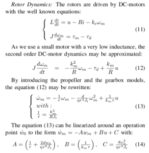
Below is what I had to go on: steps 11-14 (on the left) in the paper together with the term descriptions to the right. The one step that reads, “By introducing the propeller and the gearbox models…” is what challenged my understanding. This is where  in equation 12 becomes
  in equation 13. I did not understand how this leap was made.
Understanding of the propeller load terms…
- The
 part tells us that the propeller puts a load on the motor proportional to the square of the prop rotational speed.
- This is consistent with the last post where the NASA equations had squared airspeed difference for total force out of the prop. It makes sense that we have a squared rotational term here for torque.
- “Drag factor”, ‘d’
- Implies the drag of the air resisting the rotation of a propeller, but where can we find this?
- How did the moment of inertia go from
 to
to  ?
?- When using motors with shafts, gears, and, “loads” we want to, “refer” all of the downstream complications to the motor shaft in one, “lumped” parameter so that our problem looks like a motor spinning a disk.
- We, “lump” all the complications into an equivalent moment of inertia

- This is what represents, but how to arrive at it through the gearbox?
- This is what
- We, “lump” all the complications into an equivalent moment of inertia
- When using motors with shafts, gears, and, “loads” we want to, “refer” all of the downstream complications to the motor shaft in one, “lumped” parameter so that our problem looks like a motor spinning a disk.
- Lumped inertia term aside, a main hang-up was the cubed gear ratio in the denominator.
- Typically we apply gear ratios as a fractional step-up in torque and down in rotational speed or vice-versa.
- To see the gear ratio cubed as is confusing.
- To see the gear ratio cubed as
- Typically we apply gear ratios as a fractional step-up in torque and down in rotational speed or vice-versa.
The Eye-opener
Reading another paper helps make sense of the r3 term. The paper below uses  instead of ‘r’, so we’ll stick with the paper’s notation for a bit. My confusion resulted from not systematically applying the gearbox relationship from the motor to the propeller for the load model:


 tells us that the torque the motor sees is equal to the load torque at the propeller divided by the gear ratio (from the above gearbox equation).
This is the, “motor load” term in equation (12) from our paper above, so here we see one gear ratio term in the denominator.
Now, on the propeller-side of the gearbox we have a simple relationship for torque as a function of propeller speed squared:

But we also know that…

So it all simplifies to…


Unstuck!
The  term is our term! When we work this back through the equations we’ll get the A, B, and C terms the same as the Bouabdallah paper.
Here’s the paper that got me thinking correctly. This is an example of one to use when you’re stuck: just look at more and more source material until somebody’s treatment of a subject offers a different twist or maybe includes an additional step, diagram, or anything that helps you see it clearly.
lab2_rotary_dynamicsTotal moment of inertia as seen at the motor shaft
Let’s focus on line (3) in the PDF above so we can determine what our moment of inertia will be, referred to the motor shaft.

is simply replacing the  propeller-side torque with the

definition of torque (the F=ma for rotations about an axis).

after we use the gearbox relationships above and replace the load-side  acceleration term with the motor-side equivalent through the gearbox.
That fractional term is the propeller load inertia as the motor, “sees” it on the motor side of the gearbox. We’ve referred it directly to the motor shaft. The total inertial load on the motor is then just the sum of the motor’s and this load inertia mapped back to the motor shaft.

is then the inertia of the motor and the load referred to the motor shaft. In the case of the load, it is mapped-back to the motor shaft through the gearbox via the denominator term.
End Result of this exercise
My confusion over the term turned-out to be a blessing. It forced more time (re)working the electro-mechanical motor equations. This makes us much more confident in all the parameters and a better working knowledge of the derivation of the final differential equation and it’s terms:

The, ‘d’ term in the propeller load equation
The trick with the, ‘d’ term is it needs to multiply an  term to produce a torque.
You can find this term in “Modelling if the ETH Helicopter Laboratory Process” by Magnus Gafvert. It appears to employ comparable motors and propellers for a small helicopter test stand. Here’s Gafvert’s D term…
“Aerodynamic torque for rotor R:  (page 9, Gafvert) for what looks like a comparable hobby-sized propeller lab set-up. We can at least get started with this order-of-magnitude estimate. Those units will give us a torque (Nm) when we multiply by
  (nominal propeller speed around linearization point).
Gafvert references Mr. Weick in his paper, which is what motivated the engineering history diversion above.
Conclusion
This post has been an exercise in overcoming confusion, at least for me. It was a re-work of our motor-propeller equations with a deeper dive into the parameters of that equation.

