QuadCopter Dynamics and Controls: Ramp-Up Reading…
I started to sketch a quadrotor model myself and derive the equations of motion, but I lost confidence and figured it would be best to sample the literature first. Below is a list of papers I found online. Click the links to see the papers.
All the papers are useful, but I found the, “PID vs LQ Control Techniques Applied to an Indoor Micro Quadrotor” by Bouabdallah et al. to be a most useful reference. It is becoming my primary basis for understanding and modelling the system I need to design a controller for.
A goal here is to develop a dynamic model and controller scheme as a platform for learning and applying, “Optimal Control and Estimation” techniques.
The multi-input model can be broken into a set of independent PID servos for level flight (hover). It will be interesting to retain the coupled system in which roll, pitch, and yaw terms interact over a larger, “flight envelope” (larger roll and pitch angles) and not just small control action from level flight. It might not be necessary for much practical flying, but we’re going to follow some advanced topics for the fun of it.
The Bouabdallah paper above doesn’t jump to model simplifications and linearizations. It maintains consideration for gyroscopic effects because the focus is on a lightweight, presumably highly dynamic platform. I’m also intrigued by the, “successive linearization” concept presented.
We’re going to get a better grasp on model linearization through this exercise. We’re going to better understand how to modify the, “state transition matrix” (typically termed matrix ‘A’ for continuous control models and ‘F’ for discrete-time models). Hence the, “Linearization” paper above.
Dynamics and Controls Study Materials
I’ve enjoyed great opportunities to both study and work on mechanics, electronics, real-time control systems and supporting software for automated machines: Agricultural machine control for the most part, and some neat control systems problems in communications, sensors, and other areas.
Dynamic Modelling
One thing I really like about, modelling a dynamic system is you need to be creative to arrive at an appropriate model, or mathematical representation of a system. It is just like a scale-model in that it isn’t the, “real thing”. It is something that represents the actual system, in a form simple enough to apply some math to, but not so complicated that you can’t solve the equations into some control electronics and software.
This modelling step is my favorite part. It is the most important part. If it’s too complicated I can’t work with it. If it’s too simple, it means I’m probably ignoring something in the real world that would make any system design fail to do the job correctly. There really is not much math at this point, but a sketch and an accounting for what goes in, and what goes out: the stimuli you expect to make the system do it’s work, and also the forces of nature that want to move the system in ways you can’t always know, but need to manage somehow.
Differential Equations Comprise the Model
Because we’re dealing with dynamic systems we’re talking about differential equations to represent them. This just means an equation that describes, given where something is (it’s current state), where it is going based upon some attributes and some forces acting on it right now.
It’s kind of like this: if you know where you are standing, you know how heavy you are, and how strong your kid is who is trying to push you out the door to drive him to a friend’s house, we might know how much closer to the door you will be one second from now.
These Differential equations are the mathematical model of a dynamic system. At this point of our model they might be too complicated for us to do much with, so we might need to decide if there are terms we can ignore because they will have a small effect, or maybe we need to linearize the system by making some assumptions about the range of action (motion) we expect relative to perhaps a typical operating point.
Creativity
Proper simplification requires creativity. There are so many great examples of similar problems (especially now with the vast resources of the internet) that it is fun to borrow techniques and sometimes combine techniques from different problems to a problem at-hand. The best ideas are typically stolen.
In order to be creative and confident in our modelling of the Quad we’ll need a solid foundation. Here are some references I often revisit.
Control Systems Basics: review of the old studies
This is introductory Controls textbook.
This is introductory Discrete-time controls text that builds on the text above. Most controllers today are implemented by a digital computer that samples sensors and outputs actuator commands on a, “sampling interval”. We model this sampling and the math is a bit different (Z-transform in place of Laplace transform in the continuous time case). This is a good reference.
New Material…
I haven’t systematically studied “Optimal Control and Estimation” so after some old notes were challenging me I bought some books.
This looks like the classic text on this subject. I also found a great reference for working through the text: Weatherwax_Stengel_Notes and some MATLAB samples here
.
These last two were listed along with the Stengel book as some of the best, so I picked these up too. I’m a bit into this first one from 1970. I like some of the pre-personal-computer era books because they often tend towards math and hand calculations that promote deeper understanding. Newer texts jump to Matlab examples right away. This is great, but the old-timers did a lot with slide rules and solid understanding.
I desired to brush-up on the Lagrangian method for deriving equations of motion. I found a link to a great reference online, and I bought a couple books from the guy! His name is David Morin from Harvard, and his classical mechanics materials look excellent…he also strikes me as a fun person in his presentation of materials.
OK, enough with the books already. If you’re in school now or studied these topics before you may have similar, suitable references.
QuadCopter DC Motor(BLDC) + Propeller Dynamics
Ultimately we’ll buy Electronic Speed Controllers (ESCs) for our Quad motors. They take PWM in and produce drive voltages for brushless DC motors. Let’s jump in to understand the motor-propeller subsystem on a quadrotor.
DC Motor Modelling
You’ll find basic DC motor equations in any undergraduate dynamics textbook. I add the Bouabdallah model for the drag term, which for a simple motor would be the back-emf alone, but here we account for propeller and gearbox drag referred to the motor shaft as you can see below.
The motor-propeller speed model is non-linear. The Taylor Series expansion and evaluation about a nominal operating point is used to linearize it.
I’ll leave this post to cover derivation of the propeller-motor equation with drive voltage as the control input. This will fit within the larger quadrotor system picture later, after we build more sub-system understanding.
In the last quadcopter post we clarified the load torque of the propeller applied through the gearbox to the motor shaft. We won’t even have a gearbox but the terms in the equation needed clarification. We haven’t yet covered the main point of the propeller: LIFT! A propeller blade is just a spinning wing at each cross-sectional location.
The propeller force described in the NASA diagram in an earlier post summarizes the propeller-induced thrust force but it doesn’t tell us anything about the fluid mechanics around the prop blades.
Wings and Lift
Motivation
My MIT Fluid Mechanics professor Ain Sonin would not be happy with me if I didn’t remember a very compelling demonstration he performed to illustrate, “streamline curvature” as the lift producer. The link on his name honors his passing in 2010. He died at a young age of 72. I vividly recall his interesting lectures, impeccable sketches, approximation techniques, and his evident love of teaching. Thinking of what I learned from him, and what I should have better absorbed then, I want to cover lift here.
Propeller as Airfoil
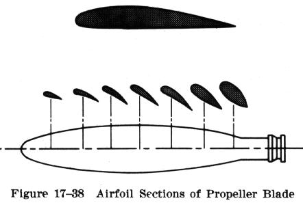
Previously, we considered the torque load as the drag on the motor. It makes sense that if we spin a propeller shaped like the example below the blunt nose and general form of the propeller requires some torque to spin it through the air. This is the drag you feel on your hand when you stick it out of your car window.
Let’s stick with the hand-out-the-window example. Whether we are actual kids or big kids, we all sometimes put our hand out the car window with our palm down. Then we tip our hand just a bit back and it feels like it wants to go up. Is this how a wing or a propeller (a spinning wing) creates sustained lift? No!
A titled hand can rise with the force of air outside the car window but we cannot sustain flight (level-flight) or produce along-axis force from spinning a propeller unless the blades produce, “streamline curvature”! This is something hard to do with your hand out the car window unless you have a very unique shape to your hand and the angles are just right.
You are likely not producing, “lift” with your hand. you are just feeling the drag on an angle and that wants to push your hand up-and-back. If it weren’t attached to your arm it would just flip backwards. If an airplane wing attempted to climb by tipping itself backwards the plane would flip back like a mattress on top of a minivan going down the highway.
It’s about, “Streamline curvature” over the top surface
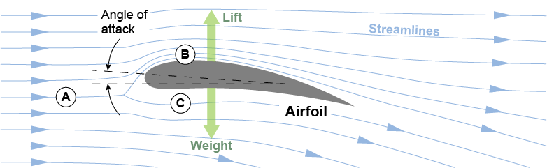
So what is really going on? In Professor Sonin’s class we were introduced to the fundamentals of Euler’s Equation, and its application in cylindrical coordinates along a, “streamline”. Streamlines are the blue lines flowing around the cross-section of a wing below. Bernoulli’s equation is what we learn to apply in basic fluid mechanics. It can be integrated from Euler’s equation. It’s handy for very many engineering problems, but Euler’s gives us a deeper level of understanding.
If you look at the cross-sections of the propeller above you can see they look like a bunch of wing cross-sections. The propeller is just a spinning wing. At any moment in time any of those propeller cross-sections above has streamlines flowing overand under similar to the simple wing diagram below. As it spins, part of the torque supplied by the motor goes into forcing these streamlines to curve around the blade. It is the nature of this curvature that gives us this, “lift” force, which we call thrust for the propeller.
For a wing, the, “weight” in the diagram is the weight of the entire plane, so the wings must produce lift to counter-act that weight, and extra lift to accelerate that weight upwards: to climb. When our propeller spins, we want it to pull a plane forward or a helicopter up (quad-copter in our case). A prop-driven airplane creates lift at the propellers to produce flight speed necessary to produce vertical lift by the wings! The prop, pulls the plane forward with, “lift” from the propellers and the plane stays aloft through, “lift” at the wings. the same principle is applied in two directions!
Our quadcopter will hover when the total lift from the four propellers matches the total weight. It will accelerate upwards or laterally when the total lift exceeds the total weight. The force we get out of a wing and a propeller is due to something you can see in the graphic above: the “streamlines” on the top (B) (the top surface of our quadrotor propellers) have more curvature than the streamlines on the bottom (C).
Euler’s Equation
The James A. Fat textbook below was in paper draft for Professor Sonin’s course at MIT 25 years ago now. Preparing for this post motivated me to (re)learn this material, so I just bought a bound copy of Fay’s book for my shelf.
Recommended Reading
We’ll gloss over considerable detail but fill a couple of gaps in the derivations that get us to, “streamline coordinates”. Otherwise, this post is just organizing references in hopes of creating a useful guide on this topic of lift as a result of, “streamline curvature”.
I can’t improve the theory relative to these expert sources. I cannot come close to the genius of Euler and the father-son Bernoulli team! I hope I can clarify it for we mere mortals.
Euler’s Equations
Euler’s Equations for inviscid flow will reveal what causes the lift once we get it into the right form. Inviscid flow is ideal, simplified flow, assumed to slip past the wing with no surface interaction (no shear, so no boundary layer, eddies, turbulence)…only the shape of the wing affects the flow, not the surface characteristics.
The Equations will reveal where the $V^2$ for the propeller speed-to-thrust relationship comes from. We glossed over this topic in the post with the NASA diagram where we saw the simplified equation with the $V^2$ term.
In the last post we resolved some confusion around the motor+gearbox+propeller model for load on the motor. We cover here the entire point of spinning the propeller: lift from the blades or aggregate thrust along the axis of the propeller.
The following PDF extracts key pages from Fay’s book (my old draft copy) that lead us to, “Euler’s Equation in Streamline Coordinates”. It includes a few pages of Bernoulli equation derivation. It is integrated from Euler’s equation along a streamline. It is a frequently applied formula.
The typically overlooked perpendicular-to-streamline (normal) Euler equation tells us about lift from an airfoil!
This tutorial by the late Professor Sonin is excellent. I enjoy his neat sketches and remember them well, as I took notes in his class and attempted to match his detail and neatness.
It’s not easy to digest the mathematical symbols, multivariable calculus, and terminology unless one has an excellent memory of their studies or practices these topics regularly. We’ll fill in some gaps below.
Cylindrical Coordinates
Although it might look daunting on its own, let’s accept Euler’s equation in cartesian (XYZ) coordinates. Then in Fay’s and Sonin’s material above we see we need cylindrical-streamline coordinates to get the equations of motion into some form that will enlighten us on this lift force we so desire.
Step-by-Step Derivation
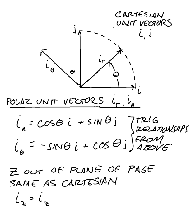
The key to deriving cylindrical coordinates is to start by representing the unit vectors relative to a Cartesian system.
Starting Point: relating (x,y) unit vectors (i,j) to polar unit vectors.
We start with radial and angular unit vectors in an X-Y plane, and we know Z in the Cartesian system is the same as Z in Cylindrical, so from the above diagram…
A big difference between cylindrical coordinates and Cartesian coordinates is the rotation of the ‘r’ and ‘$\theta$’ axes in time, as our, “fluid particle” moves in $\theta$. Hence showing $\theta$ as a function of time in the above equation.
We need derivatives of the unit vectors, and here’s what they are:
It is these moving axes that give us what look like extra terms in the cylindrical equations of motion. We get to them simply by taking derivatives of position and velocity.
We start with the position of a particle in cylindrical coordinates.
and we again replace those unit vector derivative terms and $\dot i_z=0$ to get, with a bit of rearrangement…
\begin{equation}
a = \frac{dV}{dt}=(\ddot r – r\dot \theta^2)\cdot i_r + (2\dot r \dot \theta + r\ddot \theta) \cdot i_\theta + \ddot z \cdot i_z
\end{equation}
The $2\dot r \dot \theta$ is the, “Coriolis” acceleration term and the $r\dot \theta^2$ is the “centrifugal” acceleration term for a particle. They’re nothing more than a manifestation of the rotating unit vector $i_\theta$, which we can see by following the derivation above from cartesian to polar.
Streamline Coordinates
These are just a slight twist on Cylindrical coordinates. We relate cylindrical coordinates to streamline coordinates as follows…
$i_n=-i_r$ The perpendicular-to-streamline or, “normal” to flow unit vector.
$i_s=i_\theta$ The along-path unit vector, tangent to streamline unit vector.
$i_b=i_z$ By right-hand-rule, normal to the above two unit vectors: The, “up” axis of a cylindrical system. Out-of-page axis here. No fluid dynamics along this axis.
That last denominator might look confusing but it’s just as simple as spanning a distance $ds$ with angular change $d\theta$ operating on a radius $r$.
If you now go back to the Fay PDF and accept Euler’s Equation in Cartesian coordinates on page 90-91 in the PDF above you can use the steps above to get confident with the cylindrical acceleration representation, also on page 90. From there you use the unit vector reltionships to adjust the cylindrical representation to the streamline representation and you get to Fay’s page 105 here below.
V and R being likely functions of n, integrating to estimate a pressure difference would be non-trivial. Sonin’s paper gives us a chance to solve the n-direction equation with models for Velocity and streamline radius as a function of n. See the paper to attempt this derivation for flow over a simple hill.
Fay and Sonin state that this is not a practical method for calculating a lift force. It is over-simplified, and we seldom have representations for V and R as a function of n over a range of s-vectors tangent to the flow over a wing. If we did, we’d still need to integrate them. However, this treatment tunes us into the physics of the problem. Our goal here is physical understanding, even if exact solutions elude us.
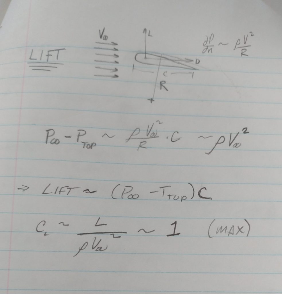
The approximation below from some 1995 Sonin lecture notes shows us what we need to know to appreciate why our prop-speed-squared ($\omega^2$) is our lift producer.
Lift lecture notes
Understanding Approximations for Lift
The n-direction equation tells us what we need to know to understand the lift generated by airfoils (thrust from propellers: spinning airfoils). As Sonin’s paper above states, “The n-direction equation states that when there is flow and the streamlines curve, the sum $p+\rho gz$ (which is constant when the fluid is static) increases in the n-direction, that is, as one moves away from the local center of curvature.”
If we imagine integrating from the wing’s surface to far above the wing the streamlines way out at our approximated infinity would have a very large radius while the airspeed is $V_\infty$.
If we just assume airspeed is $V_\infty$ everywhere (a crude approximation because we are speeding it up over the wing) but let the streamline radius get larger from top-surface radius R as we move away from the wing then we can estimate a low pressure on the top of the wing proportional to $\rho v_\infty^2$ as indicated in the lecture notes above.
Remember that if our propeller is spinning with angular velocity $\omega$. At any point along the propeller where we could take a cross-section to sketch an airfoil diagram the “V” is just the propeller rotational rate times the radius from the propeller axis to the location of our cross-section.
We now see how propeller rotational speed squared ($\omega^2$) is the variable responsible for, the “lift” generated by a propeller blade. It is proportional to a simplified, assumed freestream velocity $V^2$ at any point along the blade where we take a cross-section as above. This is a highly simplified model, but it gets us to the essence of a propeller as an airfoil.
Observe this on your next flight
Next time you land or take off in an airplane observe the flaps that extend down from the leading edge and back from the rear of the wings. They create a shorter wing curvature radius and a larger wing surface. This increases lift.
It is required because the plane is going much slower at take-off and landing than when cruising so the pressure difference across the same wing would be less at low speed.
So, the modifiable airfoil extends the flaps, creates a larger surface over which the pressure difference acts, and adds more curvature to increase the pressure difference at low airspeed. This occurs at the expense of drag, however. Given that it is only needed at low speeds, the flaps are retracted for cruising, where $ V_infty$ is higher, so we don’t need the curvature and extra area the flaps provide.
There remains that $\rho$ term for air density, and we know it is higher in the troposphere down near the ground than up at 30,000 feet and higher. We’re going to ignore this because our quadrotor is going to operate near the ground. Planes are more sensitive to “stall” (failure of the lift from wings) at high altitudes due to the rarefied (low-density) air. Airspeed and angle-of-attack are critical factors up there.
Conclusion
We now know that when our quad-rotor main controller asks our 4 motors for more-or-less speed many times per second it is the speed-squared ($\omega^2$) that gives us lift!
I hope the references above and any gap-filling explanations help convey the, “lift” phenomenon!
The equations below are from the last post, where we see we matched our Bouabdallah paper‘s equations for rotational motion.
We know some propeller input is going to be a part of the applied torque. There is going to be a set of equations for linear motion too, but let’s clarify what is going on here regarding torques about our 3 body axes. Let’s look at these equations and…
Remember Newton’s Second Law $\sum F_i=m\cdot a_i$? This tells us that the sum of the forces on a mass in the i’th direction must equal the mass of the body times the acceleration in that direction.
If we take one of the equations above and rewrite it we can recognize this familiar form, albeit in rotational nomenclature. The rightmost term is the gyroscopic effect of the entire rigid body. It tells us that if there is rotational rate about y- and z-axes a torque is induced about the X-axis. If we neglect this term you see we’d be left with $\sum_{}^{} T_x = I_x\dot\omega_x$ in simple second-law form.
It’s a little confusing, but all we’ve done is already offer one item to the, “sum-of-torques”: the gyroscopic effect resulting from the rigid body rotation. Notice when we moved the term in parenthesis to the other side it looks like an added torque now but we swapped the subtraction in parenthesis so the math is the same.
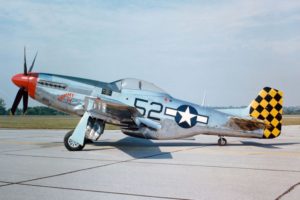
The video below to describes a phenomenon familiar to pilots, particularly pilots of powerful, “tail draggers” like the P-51 Mustang. A propeller is a large spinning disk. When we tip the plane of rotation of the propeller and pitch the airplane, torque on the body results due to this gyroscopic effect.
Imagine you are in the cockpit of the P-51, speeding down the runway (lucky you). That monster prop has a healthy angular momentum vector pointing perpendicular to the prop. Your tail is dragging until you get enough lift from your wings (due to streamline curvature, if you recall a recent post!). At some point, your tail will lift, and you’ll be parallel to the ground before your front wheels leave the ground. This looks like a quick “pitch” of, say, 15 degrees based on the photo above. Let’s say it took a second for the tail to rise as we’re nearing take-off, so the pitch rate is 15 degrees per second as the tail wheel leaves the ground.
That same pitch is pitching the plane of the spinning propeller forward, or more to the vertical. When you watch the video below and inspect the equations below you will see that this, “pitch forward” of the propeller at the above angular rate of the airplane going from dragging to level results in a gyroscopic torque about the airplane’s vertical axis: you feel the plane want to yaw (twist) so you’ll need to correct with some rudder.
The effect can be negligible
Our propellers are horizontal in the body plane, but there is a torque induced on the body that results from propeller rotation and rotation of the propeller plane about the x- and y-axis of our system, too…at least in theory. It may be negligible depending on propeller moment of inertia relative to other effects, but let’s model it anyway.
We can choose to include it or neglect it later when we perform a sensitivity analysis. This is where we can look at the rough magnitude of various effects and decide to include them in our model or cancel the terms in the equations: ignore them as too small to make a difference. We’ll do this systematically and not guess at this point. Besides, this is a neat phenomenon for us to appreciate in detail.
Video Explaining Equation Derivation
The gyroscopic effect of our propellers
The following PDF derivations arrive at the same terms as the Bouabdallah paper (equation 8). There’s a sign convention difference between the paper and these derivations, but the result is the same:
The first equation tells us that there will be a torque about our body X-axis when there is angular rate-of-change to our pitch: $\dot \phi $ (not the dot, implying pitch rate). This means our quadcopter will feel a body roll-inducing torque when it pitches. This is due to the gyroscopic effects of the 4 propellers.
The second equation tells us that there will be a torque about our body Y-axis when there is angular rate-of-change to our roll: $\dot \theta$. This means our quadcopter will feel a body pitch-inducing torque when it rolls. Again, this is due to the gyroscopic effects of the 4 propellers.
The hand calculations below arrive at the above equations following the process in the video. The video above explains how to go about the hand calculations for a single propeller.
If you expand these equations you’ll see I just performed the steps in the above video Eight times and combined the equations. We need eight steps because we have 4 propellers and we need to account for the plane-of-rotation rate-of-change about both the x- and y-axis. Rotation about the body z-axis contributes no gyroscopic effect from the propellers because it is just like twisting the axis of the propeller. The plane-of-rotation of the propeller does not change in this case so no torque is induced on the body.
We’ve now accounted for the gyroscopic effect of the rigid body rotations and the propeller rotations.
Next, we’ll add the propeller thrust components. These will be our inputs to counteract the above effects and unknown disturbances (wind) so that our quadcopter can maintain its attitude and move where we want it to go.
Finalizing Equations Of Motion: Thrust Inputs from Propellers
[latexpage]
This post explains how we determine propeller thrust and drag factors for our quadcopter project.
The last couple of posts have been working out the sum of torque on our quadcopter. A few weeks ago, we covered the gyroscopic effect of the total airframe in the “equations of motion” post.
Next, we looked at the torque induced by the gyroscopic effects of the spinning propellers in the last post.
Now we’ll consider the propeller drive inputs.
Propeller Drive Control Input
We started the, “equations of motion” with the sketch below, so we’ll use it again here as we model the command inputs from the propellers: $F_{1-4}$.
Assume the length of the arm from the center of the quadcopter to the propeller is, ‘l’ then…
$\tau_x=F_2\cdot l – F_4\cdot l$
The, ‘F’ terms are thrust forces. We know from an earlier post that this thrust from a propeller is going to be a function of propeller speed squared: $\Omega^2$:
$F = b\cdot\Omega^2$
Where ‘b’ is a “thrust factor” we need to determine. After you watch the video below you’ll understand how we get…
$b =\frac{C_t\cdot\rho\cdot D^4}{4\pi^2}$
where…
$C_t$ is an experimentally determined propeller thrust coefficient, $\rho$ is air density, and D is propeller diameter.
Our torque about the X-axis equation above becomes…
$\tau_x= bl(\Omega _2^2-\Omega _4^2)$
Torque About Body Y-axis
$\tau_y=F_1\cdot l – F_3\cdot l$
By the same logic above for the X-axis torque, this Y-axis torque becomes…
$\tau_y= bl(\Omega _1^2-\Omega _3^2)$
Torque About Body Z-axis
The torque about the Z-Axis is proportional to the squared angular velocities of the propellers. We subtract the squared counter-clockwise props from the clockwise props to lump them. The proportionality constant (the multiplier) is going to be a, “drag factor”: d.
See the video for an explanation on how we get ‘d’ from the experimentally determined, “power coefficient” for a candidate propeller.
$C_p$ is experimentally determined propeller power coefficient. $\rho$ is air density, and D is propeller diameter.
Deriving the, ‘b’ and, ‘d’ terms above
‘b’ is our thrust factor and, ‘d’ is our drag factor. They are arrived at through experimentally determined thrust and power coefficients for our propeller. We encountered the drag term earlier earlier (here) but we didn’t have insight into how it’s arrived at.
The University of Illinois and Urbana-Champaign offers an excellent resource: the UIUC Propeller Data Site. It contains wind-tunnel data for a variety of hobby-craft propellers. The following video explains how we could arrive at our drag and thrust factors through measurement.
Propeller Thrust Coefficient
Let’s estimate the thrust coefficient from the “static” data because a quadcoptor is not going to travel very fast along the propellers’ axis. A preliminary estimate for the static thrust coefficient after looking at a number of experimental data sets is…
$C_t=0.1$
From this, we can calculate ‘b’ as described above.
Propeller Drag Coefficient
Recall the motor+gearbox+propeller post. There we look at how to map the torque load of the propeller back through the gearbox to the motor shaft to get all the parameters correct in modelling the DC motor drive. In that post we have
“Aerodynamic torque for rotor R: $D = 2.91\times10^{-7} \frac{Nms^2}{rad^2}$ (page 9, Gafvert) for what looks like a comparable hobby-sized propeller lab set-up”.
We didn’t see how this term was derived though.
Confusion…
It’s a challenge (for me, at least) to find a propeller with a “drag coefficient” explicitly stated in many references.
Then I read, “While an airfoil can be characterized by relations between angle of attack, lift coefficient, and drag coefficient, a propeller can be described in terms of advance ratio, thrust coefficient, and power coefficient”here. That statement cleared some fog.
Next I found an online question from a person facing the same confusion I was experiencing. The question married the above quote to the same UIUC data I was looking at. The dialog there ultimately gets to a drag term resolved from the UIUC, “power coefficient”.
From there I made sense of it and as expressed in the video above. I derive the ‘d’ term from the experimental “power coefficient,” as explained in the video. As the video explains, I’m estimating…
$C_p=0.7$
For the APC Carbon Fiber 7.8-inch propeller, if we plug in numbers, we calculate ‘d’ as…
This is close to the number from page 9 of Gafvert above. We don’t know what specific propeller he is referencing, but we know it is in the family of these hobby propellers. We can be satisfied with this method for arriving at our drag factor from the UIUC data.
Conclusion…
We now have a good understanding of the thrust and drag factors for our propellers.
When we get into the design iterations we might try other propellers with different coefficients. We can revisit the UIUC data and compute a range of ‘b’ and ‘d’ terms as we did above. This is how we can assess propeller selection impact on the performance of our quadrotor.
Linear Quadratic Control with Reference Input
[latexpage]The last post was our introduction to the Linear Quadratic Regulator (LQR). We saw there that as we started with initial conditions or introduced a disturbance the LQR will drive the states to zero. In the simulations we saw the graphic of the copter converge on the zero state: zero roll, pitch, yaw, and respective rates all to zero.
The, “Control Law” (feedback gain K) was obtained through a solution of the matrix Ricatti equation buried in Matlab. We’ll dig into that math at some other time.
This same solution is relevant for the, “tracking” problem or servo case: when we desire the plant to be controlled to a particular set of non-zero state values.
Basic Idea
We can think of it as the reverse of our last simulated cases where we started with non-zero state initial conditions (some angles for roll, pitch, and yaw) and observed the platform converge on the zero-state attitude.
Think of this new problem as starting with zero initial conditions (a level quadcopter) and desiring the attitude, “step response” to a non-zero input.
This is a bit artificial for the quadcopter because a non-zero attitude will mean thrust in a particular lateral direction which we are ignoring at present. Our controller design will still be relevant, as this is the attitude control loop.
Ultimate Goal
Later we’ll introduce an outer position control loop that supplies the reference inputs to the attitude controller: the reference input that is the topic here. In flight it will not be a set value but a continually changing attitude reference input based on the outer position control loop’s desire to move the platform by altering the attitude and the resultant thrust vector.
Before we can illustrate how an outer position controller will command attitude to this inner attitude controller we need to understand how to introduce the reference for roll, pitch, and yaw.
The respective rates are states also, but our goal is to regulate these to zero as the attitude tracks the body angle input reference. Our reference vector will supply zero for the rate states.
Theory
Feedback Control of Dynamic Systems by Franklin, Paul, and Emami-Naeini introduces the topic via the material below. The following page copies are from a 1994 edition of their textbook.
Quadrotor Implementation
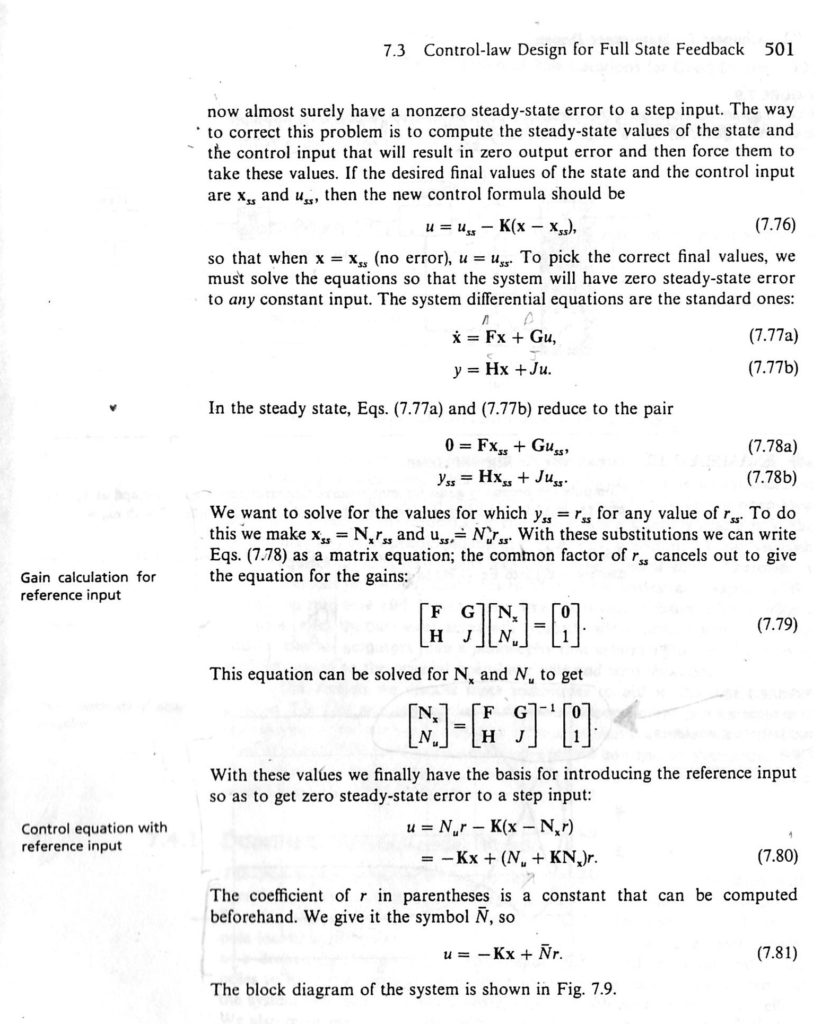
We are dealing with more states and a multi-input, multi-output (MIMO) problem. The equation to solve from the reference above is shown here with bold matrix elements representing matrices themselves.
Our ‘A‘ and ‘C‘ Matrices are 6×6. The ‘B‘ and ‘D‘ Matrices are 6×4. This results in the matrix needing an inverse being 12×10, which is non-invertible. On page 510 Stengel writes we can employ the right pseudoinverse in this case.
We can then solve for the reference gains. The resulting Nx is 6×6. The resulting Nu is 6×4. We now have the matrices we need to operate on our state reference.
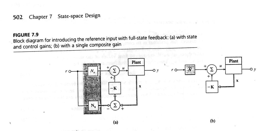
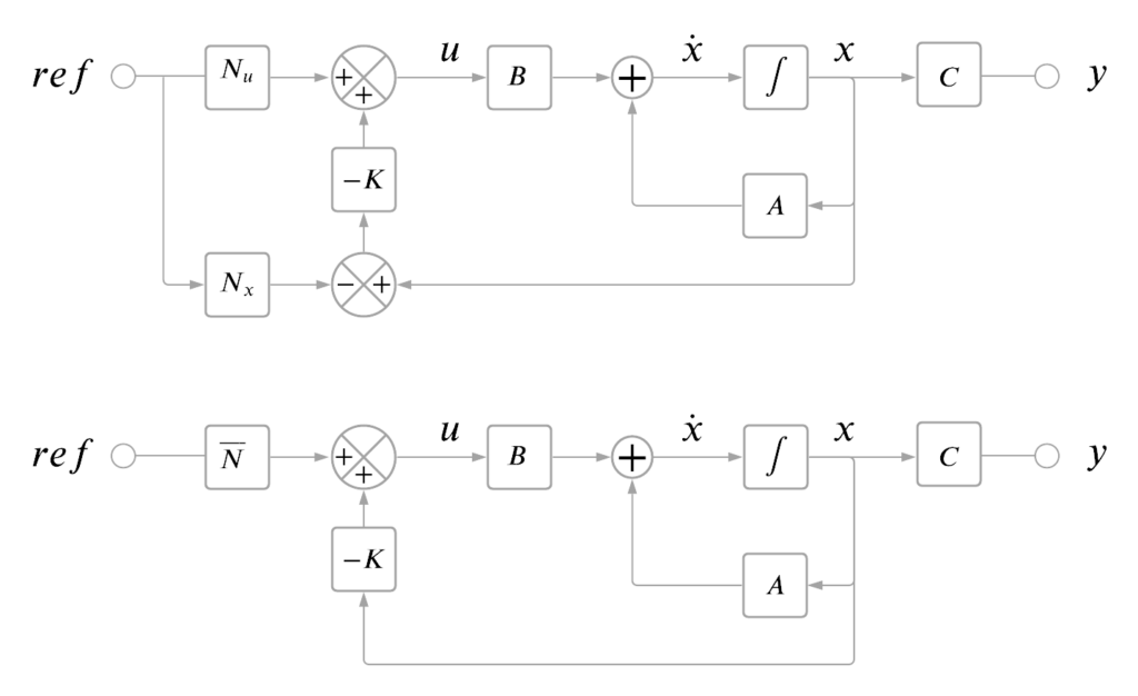
Nx and Nu are simplified into a composite gain in the second block diagram according to the reference textbook above:
\begin{equation}
\bar{N}=N_u+KN_x
\end{equation}
We’re now ready to see how the quadrotor LQ controller will track a reference input. The controller gain matrix K is from our LQR solution, so it’s the same controller.
Matlab Simulation
This Matlab script is a generalized version of the script in the last post covering the LQR simulation. In this script you will see the reference gain N is established and applied to a reference input. Yaw-axis sinusoidal reference tracking is illustrated in the following video generated by running the script.
You’ll need the same three additional files from the last post (see the matlab script section near the end).
Download the script, find yourself a Matlab seat, and explore!
Quadrotor Reference Input Tracking: a yaw-axis sinusoidal reference
Conclusion
We’ve covered how to solve for the reference input gain matrix and modified our LQR Matlab simulation script accordingly. The simple simulation shared in the video above indicates we’re stable and generally tracking the yaw sinusoid.
There’s more to do in this area: examine disturbance rejection, tracking performance, and general analysis of our LQR controller. Through this process we’d apply some performance assessment metrics and iteratively adjust our cost function weights.
We’re not yet to a real design and iteration process yet. We’re still building the tools and the understanding of how this MIMO Linear Quadratic quadcopter math works.
Happy Learning!
Maximum Thrust vs. Battery Voltage
[latexpage]
In a previous post we got the Ardupilot simulator stable running the linear-quadratic attitude controller, but we had a hack in-place for normalizing our body torque commands from Newton-meters to -1 to +1 for input to the Ardupilot motor sub-system.
Purpose
This post uses a test stand to measure maximum available thrust over a range of supply (battery) voltages in order to gain a normalizing constant we need for the output commands of our linear quadratic controller. With normalized commands we drive -1 to +1 commands into native Ardupilot motor code which in-turn drives PWM outputs to electronic speed controllers (ESCs).
Equipment
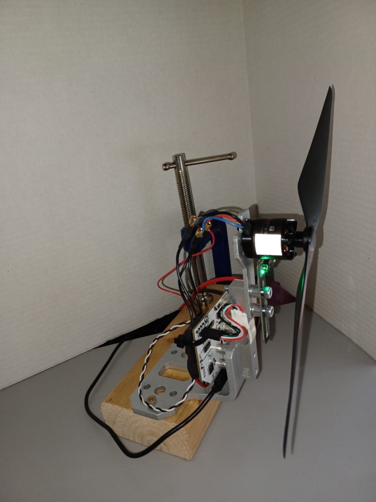
After all the modelling and equation solving for the motor-prop assembly in previous posts I’ve been wanting to take some measurements. I found a reasonably priced test stand from Tyto Robotics: their model 1520. I purchased the add-on optical speed sensor. All-in with shipping was near $200.
Here’s the 1520 on my bench with the AIR2216/880Kv motor and T1045 prop that comes with the Hexsoon EDU-450 kit. On my setup here you can see a green LED on the RPM sensor board as well as the reflective tape on the motor rotor.
Problem
In the Linear-Quadratic controller implementation within the Ardupilot Attitude Controller we’re calculating roll, pitch, yaw command outputs as Torques. Challenge is, Ardupilot motor code desires normalized roll, pitch, and yaw commands scaled -1 to +1.
Focusing on a single axis, say roll, once we have a roll torque to command on each iteration we need to cram a normalized roll (-1 to +1) into the Ardupilot motors object. From there it will result in PWM output to electronic speed controllers (ESCs) to drive the motors.
Roll torque is differential thrust from a cross-body pair of propellers multiplied by the arm length. If we divide our controllers command torque by arm length we get this differential thrust command but…
How to normalize it for the Ardupilot motors and PWM stack of code?
We need a maximum thrust
with added twist that it’s voltage-dependent as battery voltage drops during flight.
Solution
Characterize the motor-prop assembly maximum thrust as a function of battery voltage. Call it, Thrustmax.
Given Thrustmax and also run-time battery voltage sampled in real-time, scale Thrustmax down to a Thrustavailable.
Then at run-time we’ll normalize that differential thrust for roll and pitch with a divide-by Thrustavailable (first clamping the differential command to +/- Thrustavailable ). This will give us a normalized -1 to +1 roll and pitch to command the resident motors object in Ardupilot.
Yaw is different as it’s driven by propeller drag force and resultant moment induced about the craft’s center. We’ll look at that later.
Max thrust derating by battery voltage
The first plot below illustrates what to expect for thrust as our Lithium Polymer (LiPo) battery voltage drops during flight. A single LiPo charged cell is nominally 3.7 volts to 4.2V. We’ll likely use a ‘4S’ configuration (4 cells in series) for nearly 15 Volts at max charge.
I don’t yet know what a low voltage cuttoff will be. I read maybe 3.2V per cell which means our minimum operating voltage might be say 10-12V. In any case I tested with my bench supply as follows in order to produce data seen here.
Procedure
Set bench supply at 15V.
This is source voltage to the ESC driving the motor on the test stand shown above.
Step ESC from 1000 to 2100 with intervals of 100.
This results in a 1-2ms pulse to the ESC in 100 microsecond steps.
Hold each step.
Sample motor speed and torque mid-step.
When the step’s steady-state is established.
On pause after last step.
lower battery voltage.
Jump to step 2 above.
Measured Thrust over ESC range by Battery Voltage
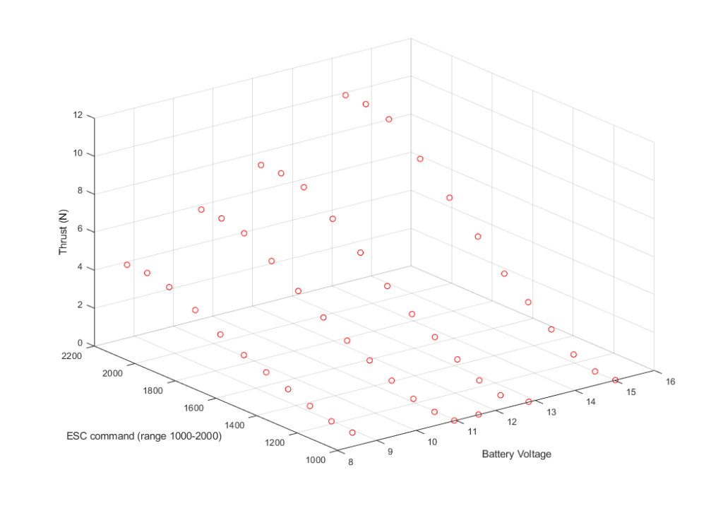
We’ll get our data off the 2-D plot below. These 3-axis plots illustrate the test runs and reveal the relationship between battery voltage, ESC command, and measured motor speed and torque.
plot: Thrust output by ESC command input over range of Battery voltage.
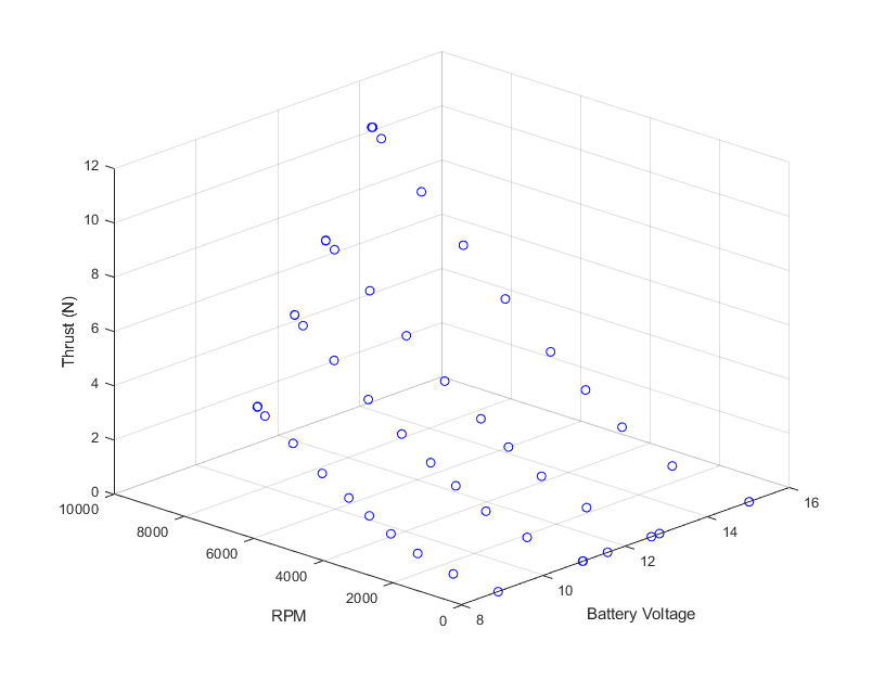
Thrust derates with voltage because the maximum RPM drops with voltage. You can see this in the following plot where we’re plotting against measured RPM instead of command. We don’t actually drive thrust, we drive motor speed, which in turn provides thrust proportional to RPM squared as described in an earlier post.
In the perspective view here you can see it’s actually RPM that is dropping with lower voltage, and consequently thrust. Thrust it our output of interest though.
plot: Thrust output vs RPM output from ESC command over range of Battery voltage.
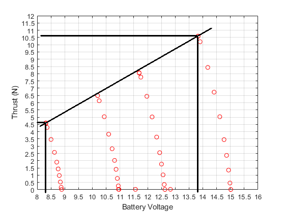
What we care about is the maximum thrust possible as a function of battery voltage. Note from the plot below how no-load battery voltage droops up to max thrust (RPM) for each step. Let’s take our voltage difference from the loaded maximum drive output for the first and last step. We’ll take the thrust difference and get our slope. It’s nicely linear.
\begin{equation} \Delta V = 13.75 – 8.25 = 5.5V \end{equation}
\begin{equation} m = \dfrac {\Delta Thrust}{\Delta V} =\dfrac{6N}{5.5V}\approx 1\dfrac{N}{V} \end{equation}
Plot: Maximum Thrust at Battery Voltage
Run-time equation for our normalizing value: Thrustavailable
The equation here will replace the normalization constants described in an earlier diagram. Our interest then was to get stable with the simulator, so we hacked-in a scheme. Here we’ll have an acurate divisor for the -1 to +1 motors input range.
We’ll confirm these results with a battery stack instead of a bench supply to finalize our numbers, but it looks like we have a tidy linear derating to apply here. We’ll calibrate somewhere near a fully-charged battery pack voltage and store these two parameters for Ardupilot:
Thrustcal (Newtons)
ThrustVcal (Volts)
ThrustSlope (Newtons per Volt)
This is unity above but we’ll store it anyway
The above run-time equation and application of these parameters will cover cases where run-time voltage is higher than the calibration voltage.
Gyroscope History: Lead Computing Gunsights
In this post we’ll dissect and simulate basic concepts embodied in early gyro instrumentation applications in combat gun sights. We’ll build a deeper understanding of gyro mechanics through this application of their first principle: output torque resulting from precession. We’ll learn some interesting history too.
The basic problem to solve is this: when we fire a ballistic projectile how can the sight compensate to have the projectile intercept a moving target down range? We desire to hold the sight on the target and not guess how much to lead it by.
The British did early work in the Mk IID sight that was also produced in the US by the Sperry Gyroscope Company as the K-14 that saw use in US fighters during WWII. Charles Stark Draper started working in the same area in 1940 out of his Instrumentation lab at MIT.
Charles Stark Draper’s Gunsight Designs
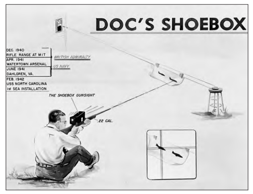
Draper’s first efforts in naval gunnery stemmed from a prototype he built in 1940 illustrated here. If some independent sensor could measure the crossing speed of the target paper, “Doc” is targeting and simultaneously know the line-of-sight of the barrel axis this independent actor could command the site in the “shoebox”.
The complicating factor is that the shoebox is the actor measuring the target crossing rate (drop rate too) by way of integrated gyroscopes. It is the, “computer” that assumes its own rates represent the target’s. This will present a problem we’ll cover below: tracking instability.
From Air Power History (SUMMER 2009 – Volume 56, Number 2), page 32 (full PDF below)
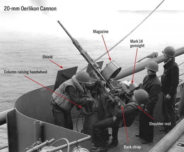
From this early, “shoe box” effort Draper designed anti-aircraft fire control systems for WWII ships. This became the Mark 14 sight manufactured by the Sperry Gyroscope Company. There’s some interesting information here.
From https://forums.spacebattles.com/threads/doc-drapers-shoebox-the-mark-14-gunsight.824442/
John H. Blakelock’s, Automatic Control of Aircraft and Missiles, Second Edition Chapter 9 and Appendix J present Draper’s later work on the A-1 air-to-air sight. Blakelock writes on page 324 that Dr. Draper, “was probably the first person to completely understand the tracking instability phenomenon and was thus able to solve this troublesome problem”. This might be generous towards, “Doc” as he was called, given the amount of varied work in this field. Click the image below for book information.
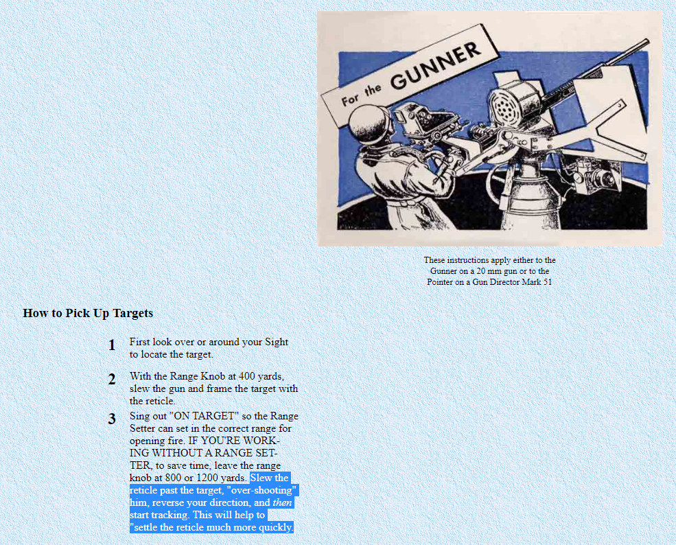
There’s a hint to this, “tracking instability” problem in training material for the Naval sight Mark 14 highlighted below. Our simulator will reveal why the Navy gave this advice. When a gunner increases slew rate of gun to catch-up to a target the pipper actually moves backwards in a manner that can confuse settling to smooth tracking. However, as you slow from ahead of a target this effect is less dramatic and easier to track to zero. We’ll make sense of this problem and identify how Draper and others mitigated the problem.
Mark 14 Naval Anti Aircraft Gun Sight Operating Advice
Draper’s A-1 Gunsight
Blakelock’s Appendix J introduces Draper’s later A-1 and A-4 air-to-air gun/rocket sight design. They were too late for WWII, but achieved some fame in the F86 Sabre vs. MIG battles over Korea in that later conflict.
The A-1 sight incorporated radar ranging. This eliminates the manual stadiametric ranging involving throttle grip twisting to close a concentric ring in the HUD on the wingspan of a target after having manually clicked the sight to specify target size. The promise of radar ranging eliminated this tedious process, but not without some growing pains as described in the article below, extracted from Air Power History (SUMMER 2009 – Volume 56, Number 2).
If you don’t read the entire article, scroll to the end and read the last paragraphs discussing the concepts of a, “heterogeneous engineer” and, “innovative departure”. These are relevant notions when attempting to gain traction when innovating in any industry or area.
Next Up…
With the above history a guide, the next post will present a simplified dynamic model we can use to investigate the, “tracking instability” problem in particular. There will be some matlab code to share so you’ll be able to play with the model yourself.
Motor-Prop Model Validation
[latexpage]
In a recent post we used the Tyto 1520 test stand to get at a maximum thrust available from our motor-prop system. We want that maximum thrust so we can normalize our LQ controller command output for the Ardupilot motor command as outlined here. The Tyto 1520 offers great value for under \$200.
While we have it set-up, let’s also have some fun validating our motor-prop equation and parameters!
Review Motor-Prop Mathematical Model
Modelling the motor-prop assembly is where the quadcopter deep-dive started way back here. Since that time we took some time to appreciate propeller fluid mechanics, and drag and thrust coefficients. We started with this…
Where, ‘V’ is DC voltage. By inspection we see this equation tells us that on the moment we apply a voltage, ‘V’ the term multiplying it is all about the motor-prop ability to spin-up while the negative term preceding on omega enforces the drag.
Another way to think about it is to observe that at some steady-state for a constant voltage input, ‘V’ if we remove V that second term becomes zero and the first term conveys spin-down of the system due to mechanical and electrical effects.
Comparing the step-response of our model using Matlab to data we collect on our test stand permits us to check some parameter assumptions to this point.
Test Stand Step Response
The Tyto RCbenchmark software permits scripting a step sequence to maximum output. The test stand is set-up to step from zero to 20%, hold, then step to 100% output. This step from spinning at 20% to maximum is our reference for model validation.
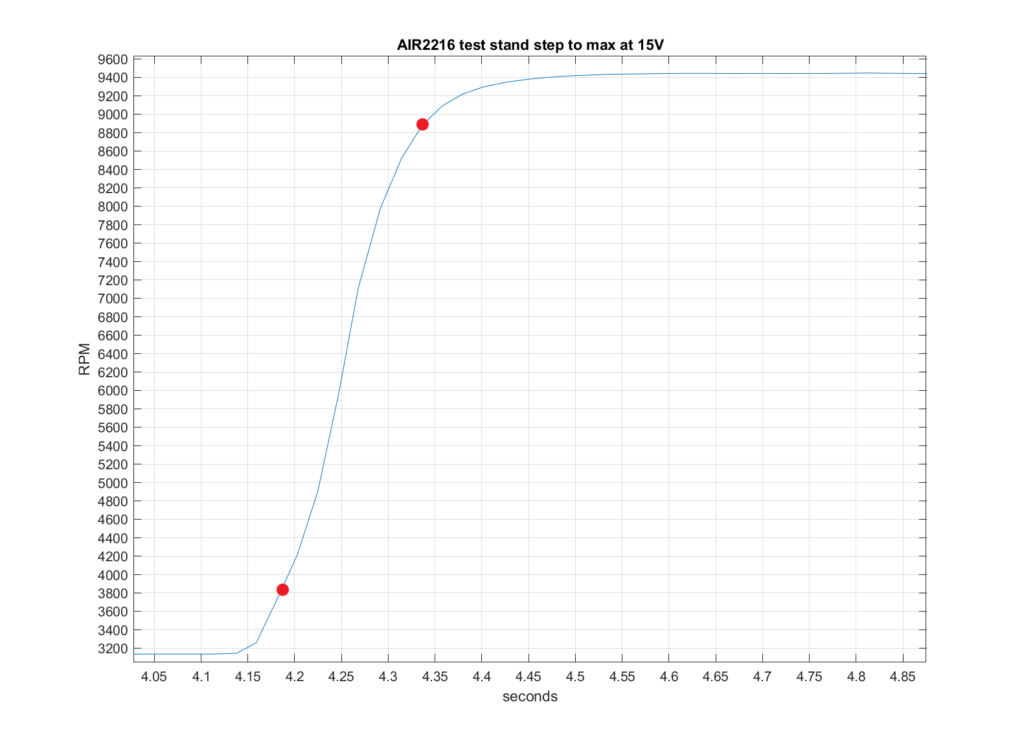
The red dots below represent the step from 10% to 90% RPM output on the transient from 20% spinning start to 100% from the electronic speed controller (ESC). This indicates a step response of 4.33-4.18= 150ms. We don’t step the prop from a dead-stop.
The start-up motor dynamics are too messy to contend with. Think of it like not wanting to model, “stiction” or what it takes to get something sliding. We want to make a step-change once sliding and avoid all the unknowns from zero. Hence we start our test stand from 20% output on the electronic speed controller, which produces near 3200RPM.
We’ll start our simulator from the same 3200 RPM too, although it doesn’t suffer from a zero start because it’s an ideal, first-order model, albeit with modelled nonlinearity in omega.
Tyto test stand output: step-response
Steady State Comparison
The first thing we want to do is check our parameters at steady-state
Set V to max test voltage = 13.85 V
This is the Maximum at steady-state with voltage droop from 15V on our test stand so…
Our largest uncertainty is likely the, ‘d’ term: the drag coefficient for our propeller. Motor resistance, ‘R’ is another uncertainty, while motor constant Km is had from 1/Kv where Kv equals the advertised 880 RPM/Volt.
Estimate Drag Factor From Test Stand Data
We measured max 9500 RPM (~1000 rad/s) above at Vmax=13.85 so to solve the above equation for our most uncertain parameter pair R and d.
ω = 1000 rad/s
V = 13.85
Km = 1/Kv = 1/880 RPM/volt = 0.011 (converting to radians and seconds)
Rearrange the Quadratic equation and solve for Rd…
Rd = 3.135 x 10⁻⁸
where
\begin{equation} d = \frac{P_{const} \rho D^5}{8\pi^3} \end{equation}
If we take motor resistance as 0.115 ohms our test stand estimate for drag factor, ‘d’ is…
d = 2.73 x 10⁻⁷
Model Drag Factor
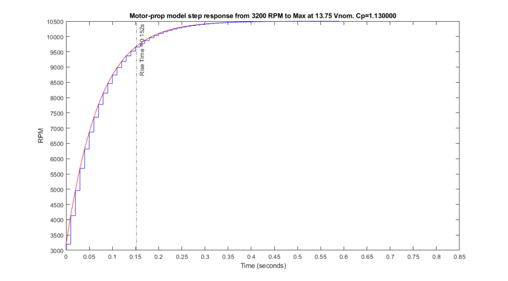
The model gives d=1.5 x 10⁻⁷ when we accept the Ardupilot SITL script assumption for propeller power coefficient Cp=1.13. Both model and above operation on test stand data assume same value for motor coil resistance of 0.115 Ohms.
For Cp=1.13 the model also produces a higher steady-state result. observing the figure below
Model Step Response with assumed Cp=1.13 from Ardupilot SITL script
Model Parameter Adjustment
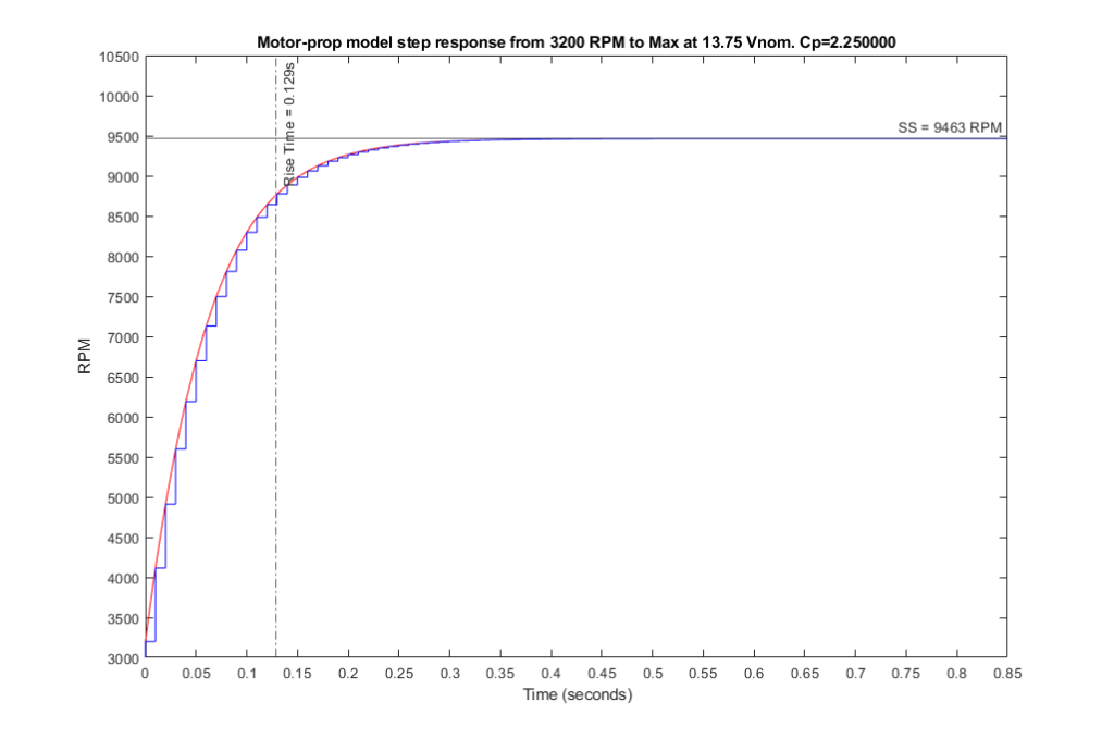
Changing the model power coefficient to Cp=2.25 yields a steady-state RPM in-line with the test stand result and a rise time that is still within 15% of the measured rise time (129ms below compared to 150 above). The test stand output plot indicates some higher-order response from zero. We don’t have those dynamics modeled. Given we have some unmodeled higher-order 129/150= 86% match on rise-time with match on steady-state is close.
Let’s conclude that our SITL Cp is too low at 1.13, and that Cp=2.25 is closer to actual than 1.13.
With model Cp=2.25 the model’s drag coefficient d = 2.97 x 10⁻⁷, within 10% of our estimate of d = 2.73 x 10⁻⁷ for the test stand.
Model Step-reponse with Cp Adjusted to better match test stand output at steady-state
Conclusion
Motor-propeller power coefficient (Cp) taken as 1.13 from the Ardupilot SITL (simulator in-the-loop) appears low. Increaing model Cp to 2.25 produces a close match on steady-state output between test stand and model for a modelled-as-same voltage step input.
Cp=2.25 yields a rise-time estimate 15% faster than the test stand. However, considering the higher-order response from intitial RPM for the test stand that we don’t have modelled this appears reasonable when examining the plots above. If the model rise from zero were higher-order like the test stand reveals this would increase the first-order simulated rise time of 129ms above, closer to the measured 150, closing the 15% error to some degree.
With Cp=2.25, a close match on steady-state output and a model simulation rise-time within 15% of measured, given our somewhat crude tools and basic methods here, let’s call the model, “validated”!